6. Manual statistical configuration
In this lesson, you will configure one statistical model for Papel branco and another for the Tissue paper family. You will then validate a preliminary forecast without yet generating an actual Demand Plan.
You will use the monthly profile created in chapter 5 with the two combinations formed in chapter 4.
1. Open the statistical configurations by combination
Open Demand Planning > Cluster-Level Configuration.
Product Cluster is the material-cluster label on this screen.
- Select Execution Profile = PD_MENSAL_TUTORIAL.
- Select Location Cluster = Default Location Cluster. It is the default location cluster and, because no more specific clusters exist, includes all registered locations.
- Select Product Cluster = Produtos acabados de papel branco.
- Wait for the saved configuration to load before editing.
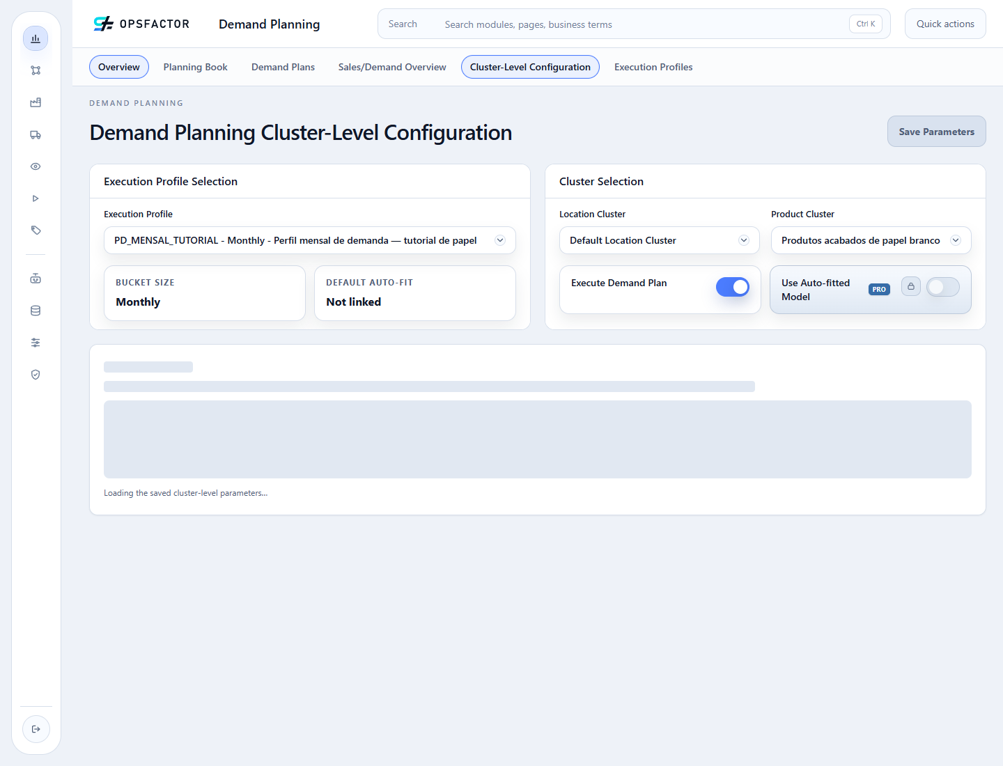
After the third selection, the platform loads the parameters saved for that combination. Only then do Forecast Split, Forecast Model Parametrization, Sales History and Coverage, and Simulation Parameters become available for editing and testing.
Statistical configurations by cluster combination
- Unit of Measure
TON: converts Sales history, loaded inKG, to the selected unit through the loaded global conversion 1 TON = 1,000 KG, allowing forecast analysis in tons. - Holt-Winters: represents monthly level, trend, and seasonality. See the internal model catalog and this conceptual material on seasonal methods.
- 1,095 historical days: covers approximately three scenario years.
- Historical Sales split: the Community model that disaggregates an aggregate forecast to material-location series.
Manual does not mean arbitrary coefficients
In Community Edition, the forecast model is selected manually, but its parameters — Alpha, Beta, and Gamma for Holt-Winters — can be calculated automatically. Fix coefficients only when a backtest, comparison criterion, and governance process support that choice.
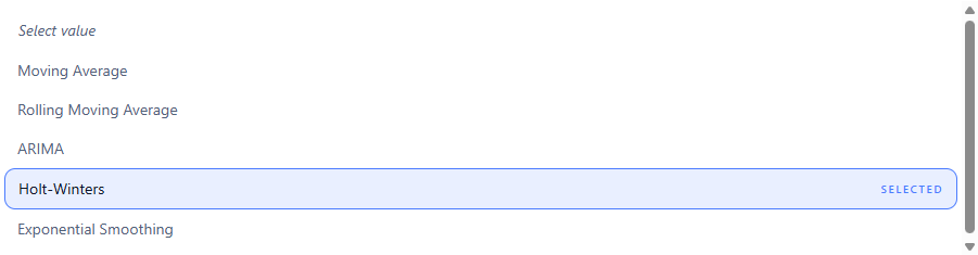
When you open Forecast Model, Community Edition presents five manual options: Moving Average, Rolling Moving Average, ARIMA, Holt-Winters, and Exponential Smoothing. Fields marked PRO remain visible to preserve the screen context, but they are locked and outside this exercise.
2. Configure the white-paper statistical model
Action required
Use white paper as the reference case: work through every section, set the fields below, and save only after reviewing the complete configuration.
Fill the Community fields:
| Section | Field | Value |
|---|---|---|
| Cluster Selection | Execute Demand Plan | on |
| Forecast Split | Split Model | Historical Sales |
| Forecast Split | Days for Top-Down Split | 1,095 |
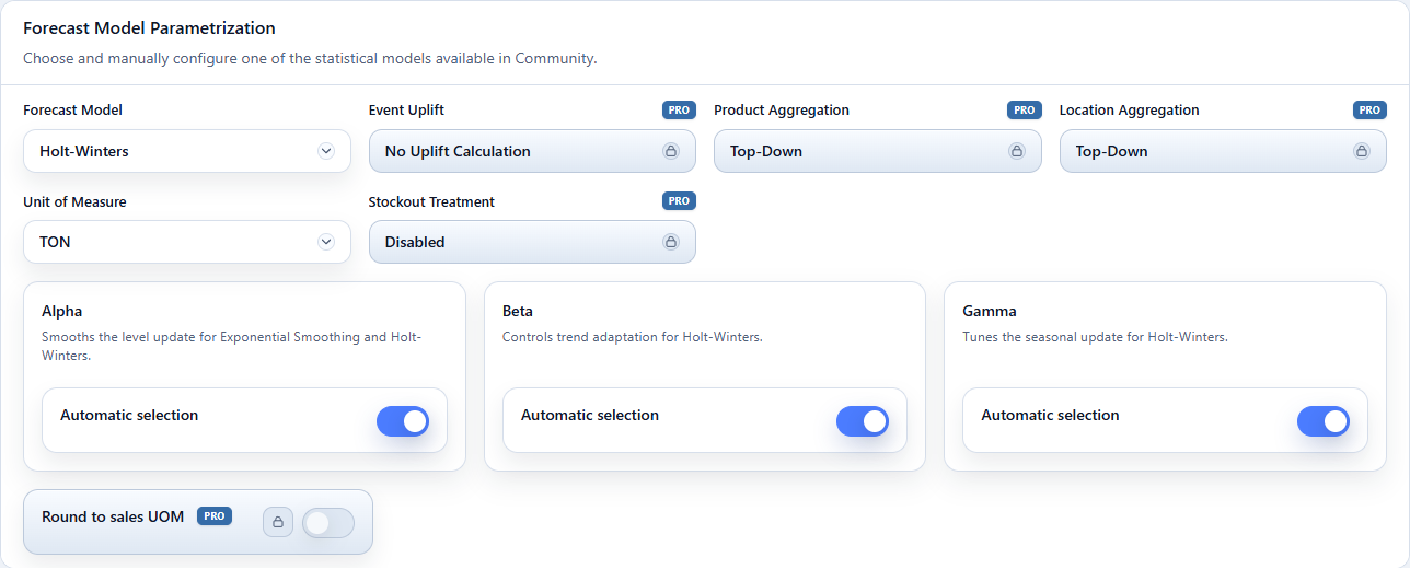
| Forecast Model Parametrization | Forecast Model | Holt-Winters |
| Forecast Model Parametrization | Unit of Measure | TON |
| Holt-Winters | Alpha, Beta, and Gamma | Automatic selection |
| Sales History and Coverage | Days of Historical Sales | 1,095 |
| Sales History and Coverage | Consider inactive DFUs | off |
| Sales History and Coverage | Generate forecast for out-of-line products | off |
With Holt-Winters selected, the Alpha, Beta, and Gamma controls appear below the model. Keep all three on Automatic selection.
Choose Save Parameters and wait for the success message.
3. Generate the white-paper forecast preview
Action required
Set the reference period to December / 2026, then choose the highlighted Generate Forecast Preview action.
- Under Reference Period, select December / 2026.
- Choose Generate Forecast Preview.
- Confirm the Forecast preview generated for 48 material-location series message.
- Under Forecast Lag (# periods) for Error Calculation, keep Lag 0 — 2026-12-31.
- Read the four KPI cards and both charts before opening the detail table.
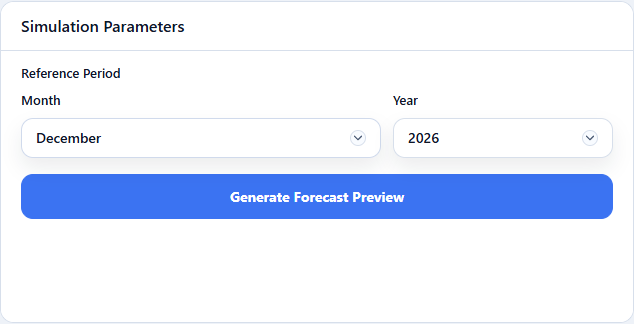

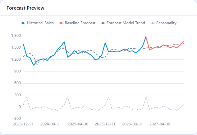
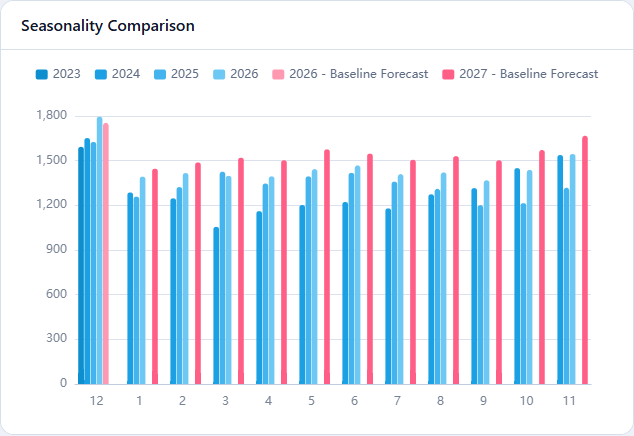
This execution runs the forecast model for a past period and enables a retrospective validation of its quality. With December / 2026 as the reference, the model uses sales through November 2026 to produce the December baseline. December actual sales do not enter forecast generation; they are used only afterward to measure the error.
The reproduced white-paper result is:
| Displayed KPI | Result | How to interpret it |
|---|---|---|
| Total Sales at Lag | 1,794.7 TON | Actual sales observed in December 2026 |
| Total Bias at Lag | -40.8 TON | The baseline was below the aggregate actual |
| % Bias at Lag | -2.3% | The aggregate deviation equals 2.3% of monthly sales |
| % MAPE at Lag | 7.0% | Aggregate absolute error across 48 material-location series |
Forecast Preview connects history to the projection and exposes the direction estimated by the model. Seasonality Comparison places the months of different years side by side so you can test whether projected seasonality remains consistent with history. The table below the charts moves from the cluster aggregate to each material-location DFU and reveals where error is concentrated.
How is the forecast distributed across individual products and customers?
A DFU (Demand Forecasting Unit) is
each material-location combination that represents the most disaggregated
level of the Demand Plan. In this tutorial, sales are recorded at six End
Client locations; each DFU combines one product with one of those locations.
A location may represent a customer or a demand region, according to its master
data. The model first calculates the aggregate forecast at cluster level (for
example, Default Location Cluster × Produtos acabados de papel branco). The
Historical Sales split then allocates each period across DFUs according to
their proportions in the configured history.
flowchart TB
  A["Cluster-level aggregate series<br/><strong>Jan 100 · Feb 120 · Mar 110 · Apr 130 TON</strong>"] --> S["Historical Sales split<br/><span style='font-size:10px;color:#64748b'>historical proportions applied to each period</span>"]
  S --> D1["DFU: Product A × North Customer · 45%<br/><strong>Jan 45 · Feb 54 · Mar 49.5 · Apr 58.5 TON</strong>"]
  S --> D2["DFU: Product A × South Customer · 35%<br/><strong>Jan 35 · Feb 42 · Mar 38.5 · Apr 45.5 TON</strong>"]
  S --> D3["DFU: Product B × North Customer · 20%<br/><strong>Jan 20 · Feb 24 · Mar 22 · Apr 26 TON</strong>"]

  classDef aggregate fill:#0b1b2e,stroke:#00bcd4,color:#ffffff,stroke-width:2px;
  classDef split fill:#e8f8f5,stroke:#00a98f,color:#0f172a,stroke-width:2px;
  classDef dfu fill:#f2efff,stroke:#7c5cff,color:#0f172a;
  class A aggregate;
  class S split;
  class D1,D2,D3 dfu;
The percentages are illustrative. The central point is that the child DFUs continue to sum to the aggregate series from which they originated. Because the proportions come from the historical sales base, planners should review the result when launches, phase-outs, or significant customer and product mix shifts occur.
For more detail, see forecast levels and clusters, statistical models, and split models.
4. Repeat the configuration for tissue
Action required
Reuse the white-paper setup as your reference. Change only the Product Cluster, confirm the same parameters, and generate tissue's own evidence.
- Change only Product Cluster to Produtos acabados de papel tissue.
- Wait for the new combination's configuration to load.
- Repeat the same model, UOM, windows, and coverage settings.
- Choose Save Parameters.
- Generate the forecast preview for December / 2026 and confirm the Forecast preview generated for 12 material-location series message.
- Check the tissue aggregate: 470.9 TON in sales, -91.8 TON bias, -19.5% bias, and
a displayed
% MAPEof 19.6%.

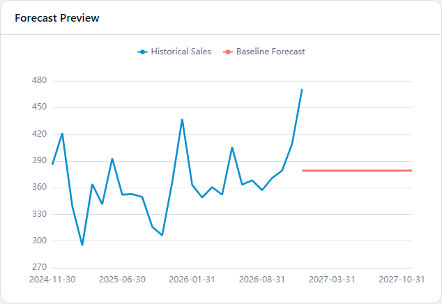
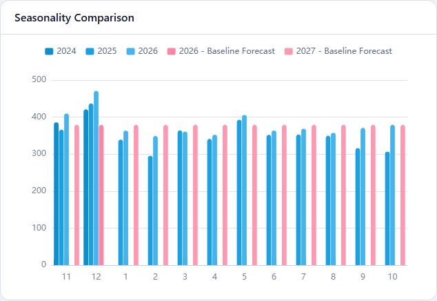
The current tissue preview underestimates December by 19.5% and has a larger error than white paper. The scenario keeps the model to teach comparison; these indicators do not constitute approval for operational forecast use.
Interpretation and governance
Both clusters start with the same model to support a controlled comparison. This does not prove Holt-Winters is the permanent winner. A mature process compares out-of-sample error, investigates bias and stability, records exceptions, and revisits parameters when demand behavior changes.
Unit failures, missing history, or empty clusters must stop validation. Never accept an all-zero preview as silent success.
Checkpoint
- monthly
PD_MENSAL_TUTORIALprofile with 12 periods saved as the general configuration; - two separate statistical configurations, one for each combination of the Default Location Cluster with the white-paper and tissue clusters;
Holt-Wintersparameters andTONUnit of Measure saved in both configurations;- Alpha, Beta, and Gamma on automatic selection;
- retrospective December 2026 previews generated and read without creating a Demand Plan;
- plan execution remains out of scope.
In the next chapter, you will use the validated configurations to generate the January 2027 Demand Plan. Return to the course map or continue to 7. Run the Demand Plan.