10. Review and export the Demand Plan
After collaboration, the planner can compare Sales and the Demand Plan, locate differences by region, and download the lines behind the result. This chapter separates those two actions: analyzing the plan and downloading its detailed dataset.
Original file and field glossary
Keep the download identical to the application export: headers, sheet names, column order, types, values and native formatting. The field tables explain the literal technical names outside the workbook. Configured descriptions and IDs are scenario data, not translations applied after download.
1. Open Sales/Demand Overview
1. In the sidebar, select the Demand Planning icon.

2. In Visibility, select Sales/Demand Overview.
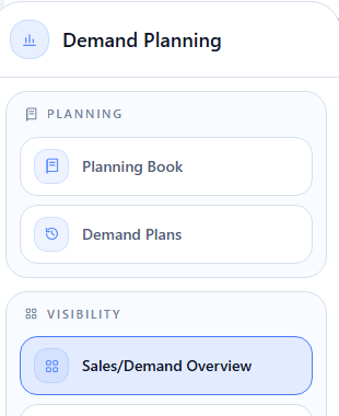
On the open page, make these selections:
- under Demand plan version, choose Plano de demanda — janeiro de 2027 — Community 2026.09.22 PT;
- under Unit of measure, select
TON; - under Historical horizon, enter
12; - keep Detail level set to Detailed by material and location;
- scroll to the end of the filters and click Open overview.
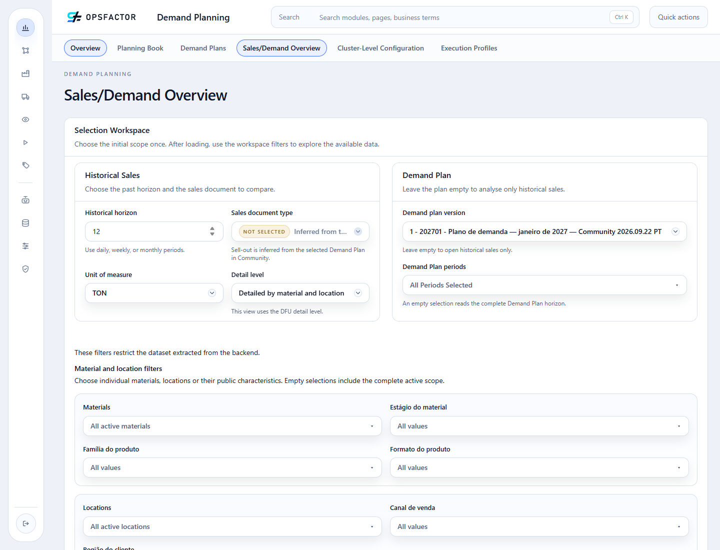
Sales document type is filled from the selected plan and does not require another choice in this step.
Action to perform
Select the scenario, TON, 12 periods, and material-location detail;
then open the overview.
2. Read the indicators and organize Pivot Analysis
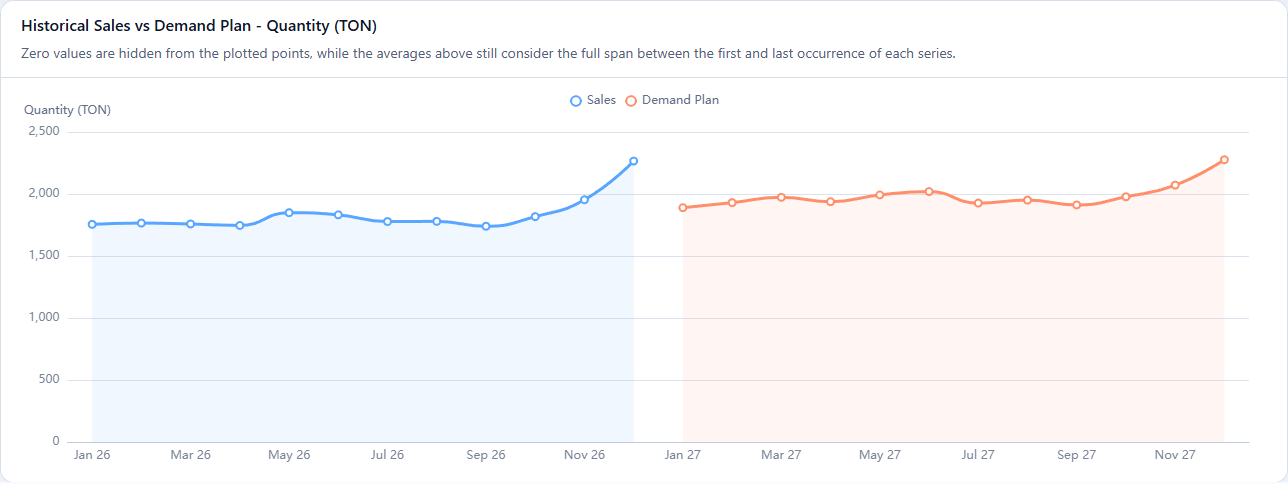
The workspace shows local filters, the historical average, and the Demand Plan average. The screenshot shows rounded monthly averages of 1,837 TON for history and 1,988 TON for the plan. The same workspace contains the chart with January–December 2026 Sales and the January–December 2027 Demand Plan.

In Pivot Analysis, open the configuration panel and build the regional view:
- keep Series under Group By;
- also add Customer Region under Group By;
- keep Period under Split By.
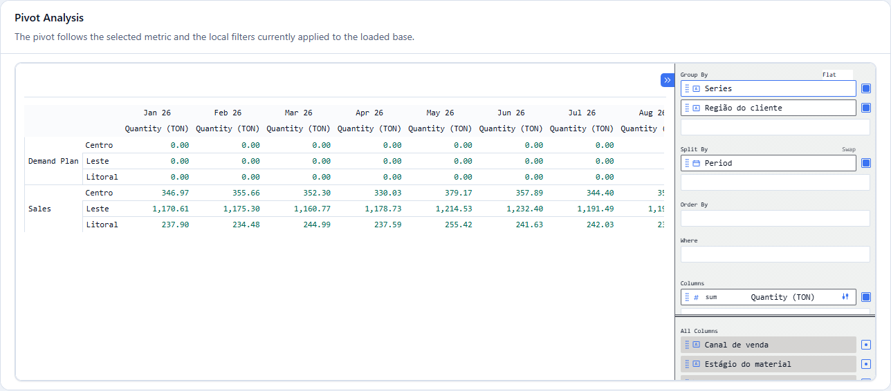
The first grouping separates Demand Plan and Sales; the second expands each series by Customer Region. Months remain in columns because Period is under Split By. This lets the planner compare Central, Coastal, and East without losing the monthly sequence.
How to interpret it
A higher plan average is a signal to investigate, not a conclusion. Compare regions in the pivot and use material and location filters to locate the source of the difference.
The visible columns in the screenshot belong to 2026: Demand Plan is zero because the plan starts in 2027. Scroll the pivot horizontally to the 2027 months to read the plan; the historical columns do not indicate a missing forecast.
3. Open the Demand Plan in Planning Data
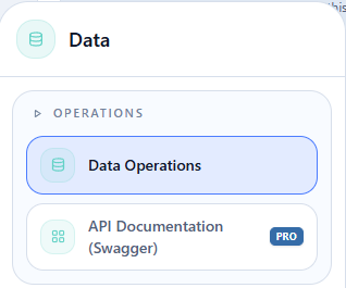
1. In the sidebar, select the Data icon.

2. In Operations, select Data Operations.
On the open page, follow the catalog without skipping levels:
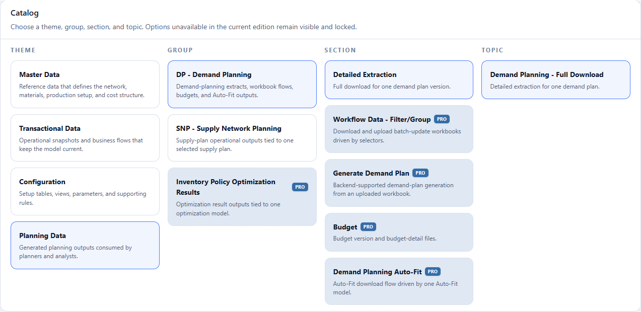
- select the Planning Data theme;
- select the DP - Demand Planning group;
- select the Detailed Extraction section;
- select the Demand Planning - Full Download topic.
4. Download the XLSX
In the Download operation:
- under Export Scope, select Complete dataset;
- under Demand Plan, select the scenario generated in chapter 7;
- keep the XLSX format;
- click Download as.
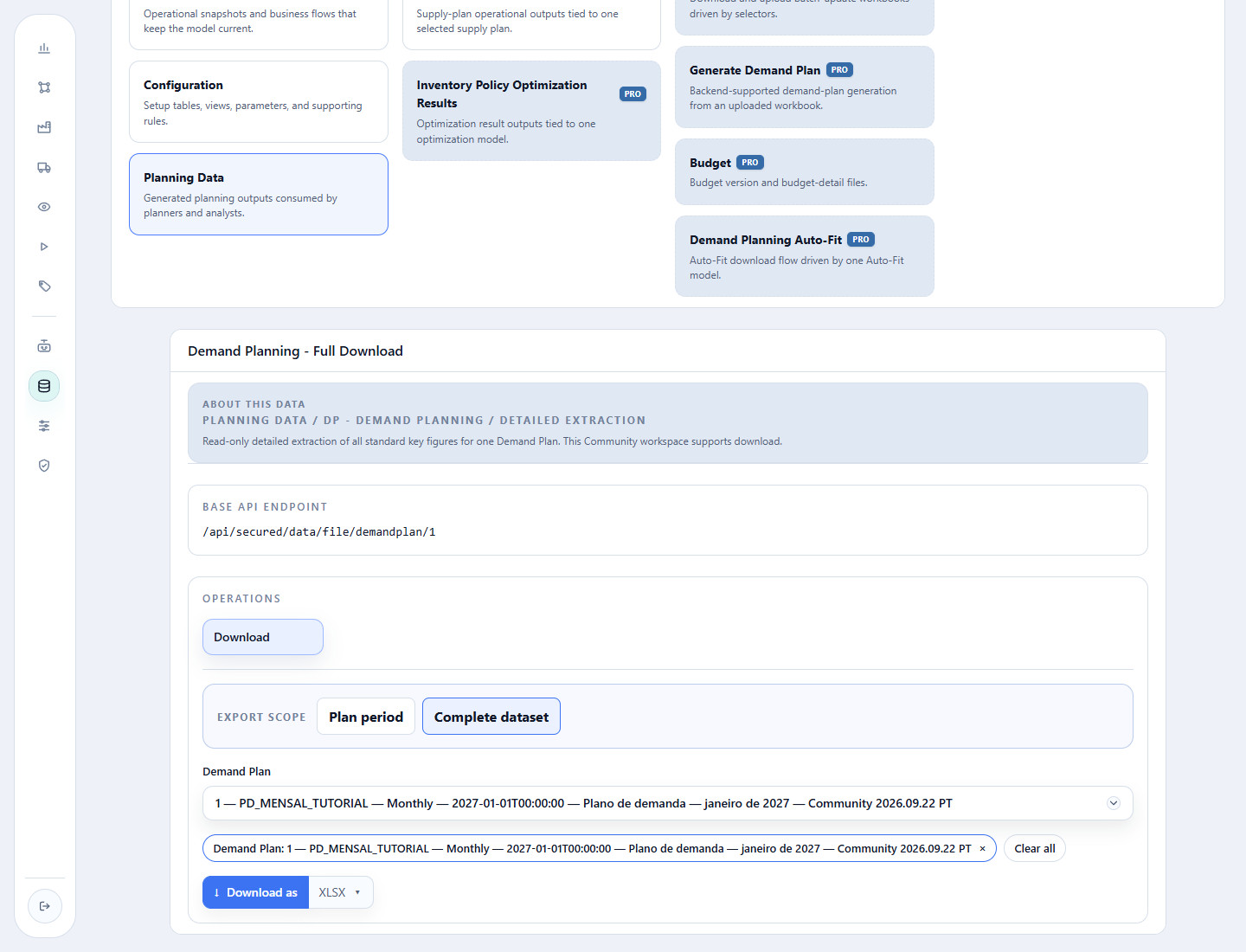
The download uses /api/secured/data/file/demandplan/{demandPlanId} and creates
a workbook with 720 data rows: 60 material-location combinations across 12
months.
5. Read the workbook
Read-only excerpt from the original XLSX: sheet Data, 720 data rows. The first five rows below preserve the exported headers and values; webpage presentation does not change the file.
| Editable (changing will result in the creation of another record in the database) | Editable (changing will result in the creation of another record in the database) | Editable (changing will result in the creation of another record in the database) | Ignored on upload | Editable | Editable | Editable | Editable |
|---|---|---|---|---|---|---|---|
| Location Id | Product Id | Date (represents the end of each period : month/week/day) | Unit of Measure Id | Baseline Quantity | New Products Quantity | Uplift Quantity | Adjustment Quantity |
| REGIONAL_CENTRO_DIRETO | PA_BRANCO_75_A4_100 | 2027-01-31T23:59:59 | TON | 9.641457211332794 | 0 | 0 | 0 |
| REGIONAL_CENTRO_DIRETO | PA_BRANCO_75_A4_100 | 2027-02-28T23:59:59 | TON | 9.903106503861773 | 0 | 0 | 0 |
| REGIONAL_CENTRO_DIRETO | PA_BRANCO_75_A4_100 | 2027-03-31T23:59:59 | TON | 10.197754641973477 | 0 | 0 | 0 |
| REGIONAL_CENTRO_DIRETO | PA_BRANCO_75_A4_100 | 2027-04-30T23:59:59 | TON | 9.96174099706871 | 0 | 0 | 0 |
| REGIONAL_CENTRO_DIRETO | PA_BRANCO_75_A4_100 | 2027-05-31T23:59:59 | TON | 10.317966386863628 | 0 | 0 | 0 |
The first four columns identify location, material, period end, and UOM. Quantities have the following meaning in Community:
- Baseline Quantity: the statistical forecast generated by the execution;
- Adjustment Quantity: the change entered through Planning Book collaboration;
- New Products Quantity and Uplift Quantity: remain zero in Community;
- final plan: Baseline Quantity + Adjustment Quantity.
For PA_COPIA_A4 / REGIONAL_CENTRO_DIRETO, the previous exercise records
+1.00 TON in January, +1.50 TON in February, and -0.50 TON in March
2027. Added to their baselines, they yield 9.61, 10.35, and 8.61 TON,
respectively, when rounded to two decimal places.
Download the tutorial scenario XLSX
Action to perform
Open the workbook and filter Material to PA_COPIA_A4 and Location
to REGIONAL_CENTRO_DIRETO. Locate January, February, and March 2027.
Check all three deltas and add Baseline and Adjustment to reconcile
9.61, 10.35, and 8.61 TON. Retain baseline precision in the
calculation and round only when comparing with the screen.
Completion criterion
Complete this chapter when the pivot shows Sales and Demand Plan by Customer Region and the XLSX is reconciled to 720 rows and the three saved adjustments.
Return to the collaborative adjustments, or continue with production and capacity data.