4. Propose DCs with barycenter analysis
What you will build
Filter DC-only demand and inspect candidate coordinates and distances.
Before starting
Use the study demand and customer locations already classified by service rule. The previous chapter’s network versions will be used to assess selected candidates.
Barycenter analysis generates candidate locations. It is a geographic proposal step; the full comparison of facility opening and operation takes place in network optimization.
Select the market and run the first analysis
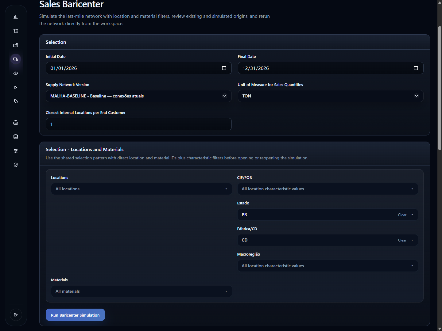
- Open Sales Baricenter. In Selection, enter the study's Initial Date and Final Date, select Supply Network Version, and choose TON in Unit of Measure for Sales Quantities for this scenario. The annual scope uses 2026-01-01 through 2026-12-31.
- In Selection - Locations and Materials, filter only customer locations served exclusively through a DC and the study region. Include the relevant CIF/FOB shares; exclude the plant-or-DC segment and reference municipalities without their own demand. Check scoped volume before interpreting any proposed position.
- Set Closest Internal Locations per End Customer. This field controls how many nearby origins are associated with each customer; it does not define how many new DCs will be proposed.
- Click Run Baricenter Simulation. Check Existing Locations and which current facilities are included in the geographic comparison.
For the demonstrated run, select MALHA-BASELINE, Estado = PR, and Fábrica/CD = CD. Leave CIF/FOB unrestricted to include both shares; Materials also remains unfiltered. The closest-origin count is 1.
Compare 1, 2, 3, or N candidates
- In Simulated Locations, use Create New to add one candidate row. An alternative with three new locations needs three candidate rows, rather than merely three nearby origins per customer.
- Check the selected existing facilities and candidate rows. Click Run New Simulation to recalculate. After changing filters or configuration, run it again before using the result.
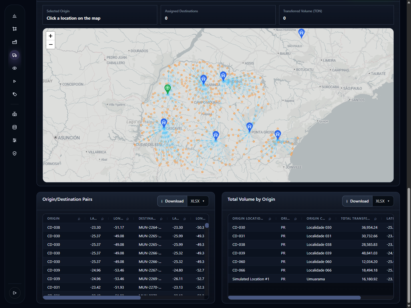
- Examine Last Mile Network with Simulated Locations and the Simulated Locations table. Check each proposal's latitude and longitude.
- In Origin/Destination Pairs, check the proposed origin, customer, proximity, and distance in kilometers. Use Download to export pairs; in Total Volume by Origin, check the volume assigned to each origin. These records support the connections in the next chapter.
- Repeat with two, three, or N rows in Simulated Locations, keeping the market, period, and unit unchanged. Record quantities and assumptions for each alternative so the comparison can be reproduced.
- Review physical and commercial feasibility, capacity, and facility cost. A suggested coordinate does not establish the availability of a property.
Check the calculated proposal
The following result retains seven selected existing locations and includes one candidate. Simulated Locations returns Umuarama, PR, latitude -23.7656, and longitude -53.3201. Check these values before preparing the new location's master record.
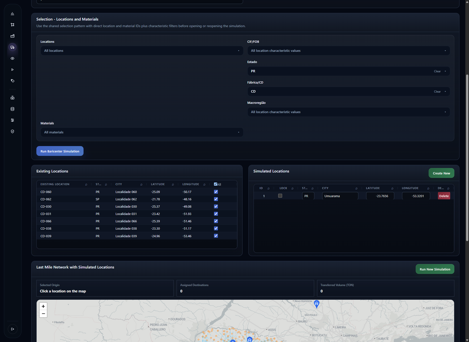
The map shows scoped origins and customers. In Total Volume by Origin, Simulated Location #1 shows 16,180.92 TON (rounded on screen). This volume belongs to the barycenter's geographic assignment; subsequent economic optimization still determines the operating flows.
Check candidate-to-customer distances
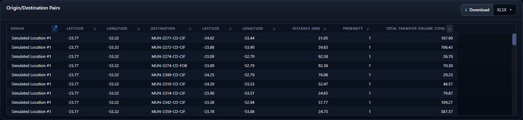
In Origin/Destination Pairs, open the Origin column filter and search
for Simulated Location #1. Scroll horizontally to Distance (km) and
Proximity. The sample shows 31.05 km for MUN-2271-CD-CIF and
59.83 km for MUN-2272-CD-CIF, both with proximity 1. Distance is
already part of the output; it does not need to be estimated visually from
the map when preparing these connections.
The capture below frames the actual table. Coordinates are rounded in this display; preserve the proposal's original precision in location master data, rather than copying the shortened latitude/longitude from the grid.
Filtering DC-only customers keeps the proposal aligned with the service problem. Including all industrial demand supplied directly by plants can move a candidate toward a market that does not require a DC.
Repeat with two and three candidates
Starting from the first proposal, click Create New once and run Run New Simulation to calculate two candidates. This scope proposes Umuarama and São Miguel do Iguaçu. Add another row and run again: the three-candidate alternative adds Verê. Keep the same filters and selection of existing facilities.
| Proposal in the three-candidate alternative | Latitude | Longitude |
|---|---|---|
| Umuarama, PR | -23.7656 | -53.3201 |
| São Miguel do Iguaçu, PR | -25.3492 | -54.2405 |
| Verê, PR | -25.8772 | -52.9051 |
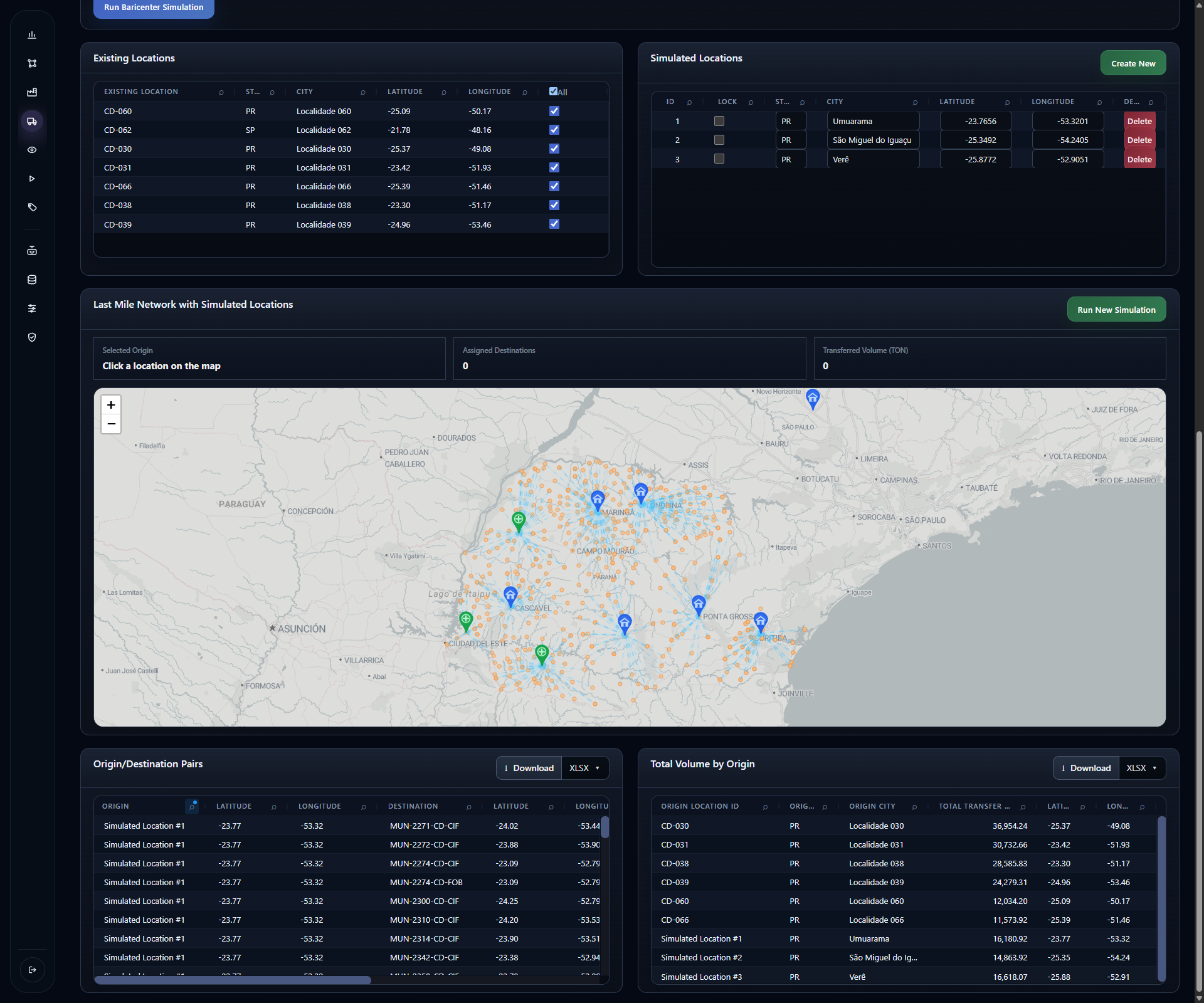
For N candidate locations in the same run, maintain N candidate rows and recalculate. The number of geographic origins and the volume assigned to each do not determine how many DCs should open: costs, connections, and constraints will be evaluated by optimization.
The rest of this training uses only the Umuarama proposal, registered
as CD-NOVO-001. São Miguel do Iguaçu and Verê remain proposals from this
analysis; they were not added to the demonstrated brownfield network.
Check before continuing
The scope includes only DC-exclusive demand. Each selected candidate has checked coordinates and proximity pairs. Proposals still need to become master data in the next chapter.
Previous: 3. Prepare the baseline and network versions.