7. Run and compare results
What you will build
Reconcile fulfillment, flows, and P&L and extract the data supporting the decision.
Before starting
Use saved profiles and check that demand, horizon, prices, costs, and units support a comparable analysis.
Run the baseline first. Before comparing scenarios, check demand fulfillment, current flows, and recognized costs. Then keep demand, prices, horizon, and units identical across scenarios, changing only the assumptions the comparison is intended to evaluate.
Use reports such as P&L to compare revenue, production costs, transfer freight, delivery freight, DC costs, and economic results. Also retain fulfillment, active constraints, and selected facilities: savings obtained by leaving demand unserved are not an equivalent comparison.
Datasets can be extracted through Data > Data Operations by selecting the topic and the Download operation. Record the network version, profile, demand, horizon, and capacity assumptions with each result so the analysis can be reproduced.
| Check | Acceptance criterion |
|---|---|
| Segmentation | Splits sum to original demand by material, municipality, and period |
| Eligibility | DC-only customers do not receive direct plant deliveries |
| Freight | FOB delivery zero; internal transfers and CIF delivery correctly valued |
| Candidates | Coordinates, distances, and inbound/outbound connections checked |
| Profile | Complete regional scope; fixed and optional facilities distinguished |
| Comparison | Same demand and economic basis; capacity differences disclosed |
| Result | Fulfillment, flows, and P&L reconciled before recommending an opening |
Economic basis of the example
The demonstrated scenario has transportation and facility costs but no registered selling prices. Read this chapter's comparison as a comparison of modeled logistics costs and demand fulfillment. The P&L report exposes those components; missing revenue values do not mean that actual revenue is zero and cannot support a margin calculation. The production routings used also lack industrial-cost components that would allow that part of the P&L to be reconciled. The study therefore compares transfer freight, delivery freight, and location fixed costs; it does not present industrial cost as zero or claim a complete economic cost-to-serve.
No prices were created to complete the example. For a margin analysis, include prices and the remaining economic components, check their effective dates and coverage, and rerun the scenarios. The new candidate's zero activation cost also excludes CAPEX from this exercise: potential operating savings alone are not an investment recommendation.
Keep the comparison scope unchanged
This training's operational comparison uses the Paraná scope, including the origins required to supply it. Run the baseline, flexible current network, and brownfield over that same scope. The overall profiles in chapter 6 organize the model; regional results do not establish that the national network has been executed. Before extending it, complete and check freight and distance coverage for the other regions.
Barycenter analysis reads the selected history; Supply Plan uses the Demand Plan selected at execution. Their totals need not coincide when projections or returns treatment differ. Comparability here requires the same future demand data across the three network alternatives.
Select the execution scenario
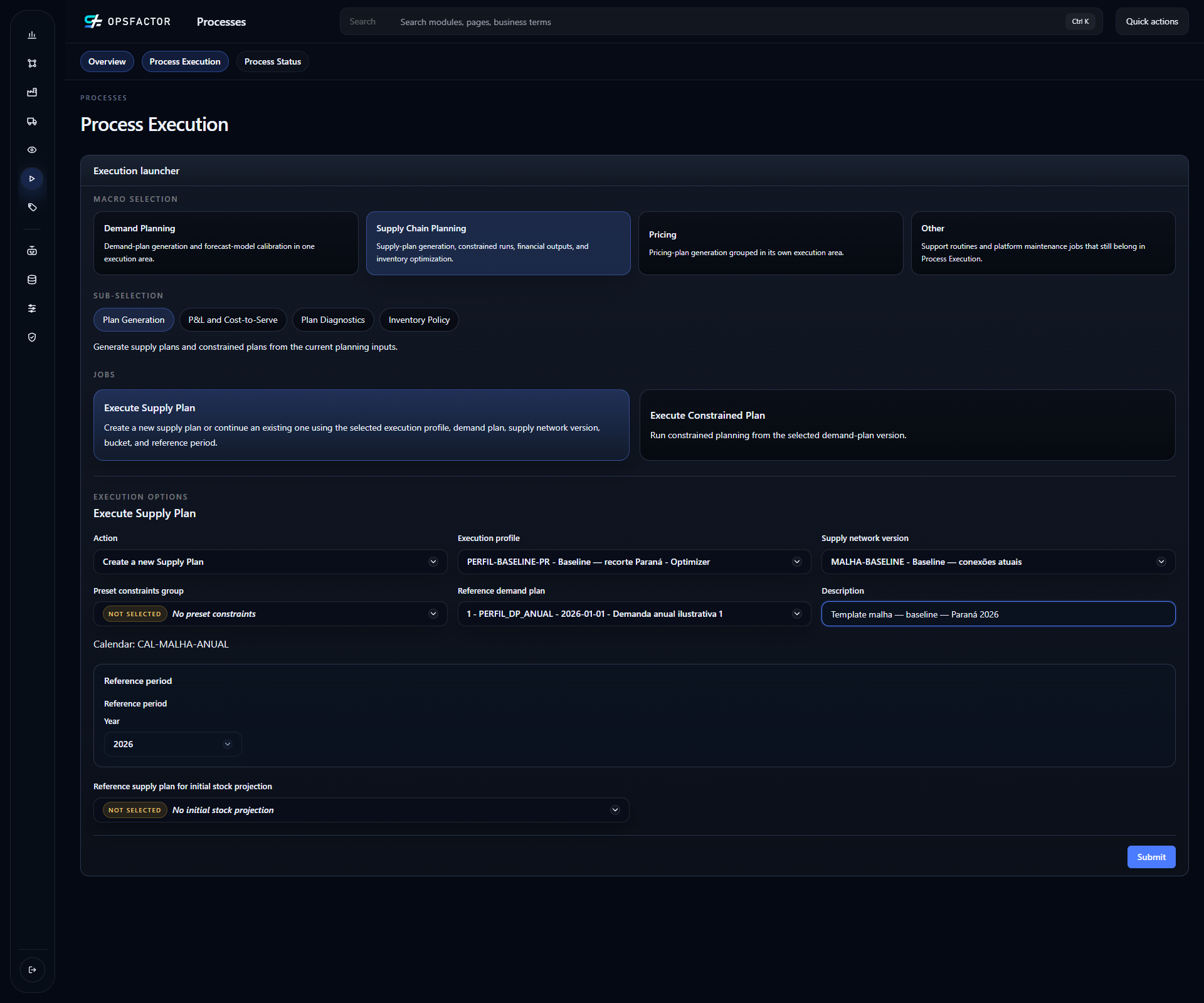
In Processes > Process Execution, open Supply Chain Planning > Plan Generation > Execute Supply Plan. Choose to create a new plan and select the profile, network version, and annual Demand Plan. Check the one-period annual calendar displayed by the page and use 2026 as the reference, corresponding to a 2026-01-01 plan start.
Use the following combinations from the demonstration scenario:
| Comparison | Profile | Network version |
|---|---|---|
| Regional baseline | PERFIL-BASELINE-PR |
MALHA-BASELINE |
| Regional flexible current network | PERFIL-FLEXIVEL-PR |
MALHA-FLEXIVEL |
| Regional brownfield | PERFIL-ABERTURA |
MALHA-BROWNFIELD |
For all three runs, select Demand Plan 1 — Demanda anual ilustrativa 1, calendar CAL-MALHA-ANUAL, and start 2026-01-01. A supply-plan number will be assigned to each run; check it before extracting results.
Keep the same start, calendar, and demand when comparing scenarios. A date change can select a different freight-table validity period or other master data, even when the network name stays the same.
The screenshot shows the completed form for the regional baseline. Check Action = Create a new Supply Plan, the three scenario selectors, and Reference period > Year = 2026 before clicking Submit. Then follow the task in Process Status; this configuration screen does not establish that the run has completed.
Run and preserve the comparison
- Run the regional baseline profile and follow processing until the plan is available. Open the persisted result and confirm profile, network, demand, and period. An accepted submission does not establish a completed run.
- Reconcile baseline service and flows with the control prepared in chapter 3. Check one CIF delivery, one FOB delivery, and one internal transfer before interpreting the comparison economically.
- Run the regional flexible-current-network profile with the same demand and cost basis. Compare the gain from changing permitted origins while keeping any capacity differences explicit.
- Run profiles with candidates and record which facilities were selected. Check inbound and outbound volumes, demand service, and the activation cost considered. Compare each regional study with a baseline of matching scope.
- Open the P&L for comparable plans and examine the result components. Lower delivery freight may come with higher transfer or DC costs; the decision must consider the combined economic effect.
- Export the report and extract the required datasets through Data. Reopen the files and check plan, period, unit, record count, and totals. Preserve network and profile identifiers so another person can reproduce the analysis.
When presenting a recommendation, connect each alternative to its service level, selected facilities, economic result, and capacity assumptions. If the baseline does not reconcile, resolve that difference before treating a scenario delta as a benefit of the new network.
The barycenter proposal does not require a DC to open. Optimization may
keep CD-NOVO-001 closed if its combination of fixed cost, inbound supply,
and delivery does not justify activation. Even with zero activation cost,
the candidate's operating cost participates in the decision. Record the
observed choice and examine its flows and costs; do not change assumptions
merely to obtain a favorable opening result.
Interpret fulfillment before comparing costs
The baseline and flexible runs in this example do not fulfill all demand. The baseline explanation distinguishes missing supply alternatives (SUPPLY_ALTERNATIVES) from objective-function decisions (OBJECTIVE_FUNCTION_COST_STRUCTURE). In the flexible network, unfulfilled demand was attributed to the latter. Capacity constraints are disabled in this study; do not attribute this shortfall to a capacity limitation.
Fixed Value / Unit Sold can make the model prefer leaving demand unfulfilled when the benefit defined in its objective does not compensate for the costs considered. This differs from a physical lack of an origin or transportation option and does not represent an observed commercial price. If the service target requires different fulfillment, review the objective and fulfillment rules before running another comparison.
Always present demand volume, fulfilled volume, and shortfall alongside costs. A raw cost difference between plans with different fulfillment does not, by itself, demonstrate savings for providing the same service.
Generate and open the P&L
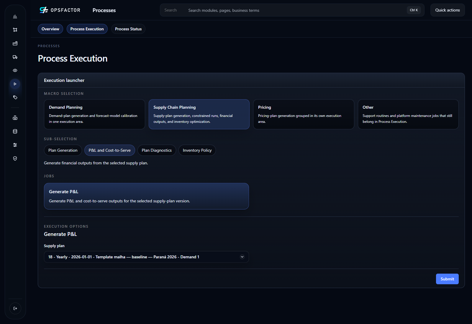
After persisting each Supply Plan, return to Processes > Process Execution and select Supply Chain Planning > P&L and Cost-to-Serve > Generate P&L. Choose the plan you just checked and run financial generation. Wait for it to finish in Process Status before opening the report. Supply Plan execution and P&L generation are separate steps in this workflow.
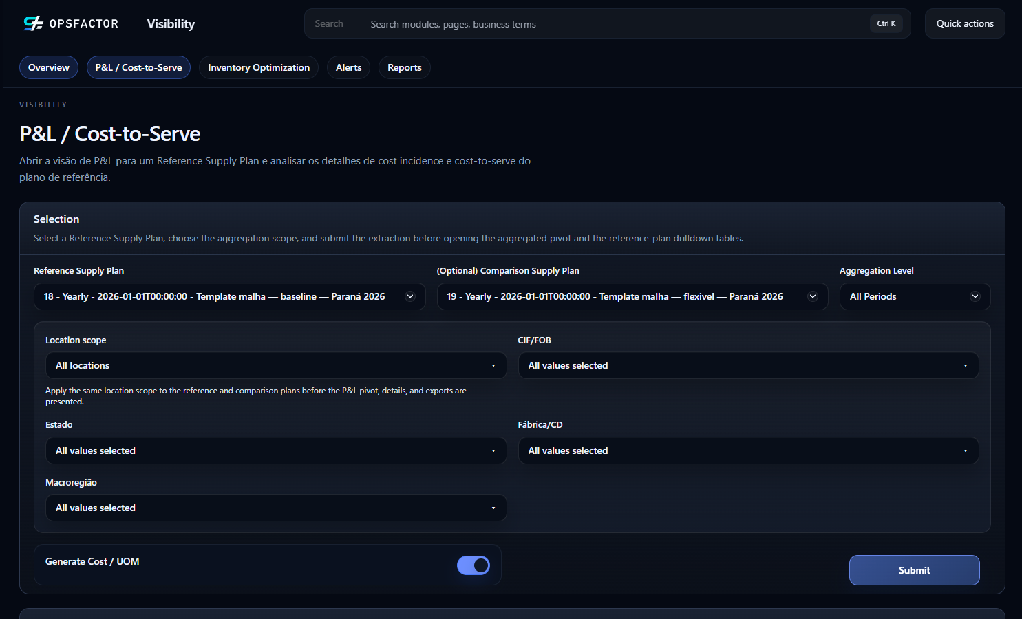
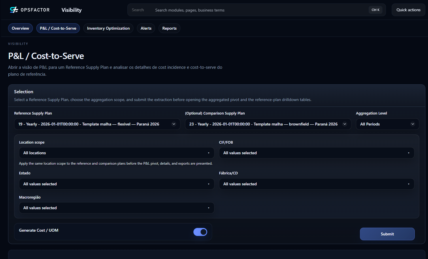
On P&L / Cost-to-Serve, select the baseline in Reference Supply Plan and the alternative in (Optional) Comparison Supply Plan. Use the same Aggregation Level, keeping Location scope and material filters consistent across plans. Click Submit to load the comparison. Start with the complete scope of the regional plans: filtering only clients can hide amounts that remain at the originating plant or DC.
The illustrated comparison uses 18 as reference and 19 as alternative, with Aggregation Level = All Periods and Location scope = All locations. Characteristic filters retain all values. These plans were already executed within the regional scope; the report does not need to exclude enabled origins outside the state again.
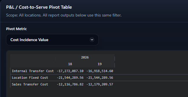
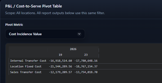
In the pivot, select Pivot Metric = Cost Incidence Value. The native capture below shows the extracted result: Internal Transfer Cost is internal freight, Location Fixed Cost is facility fixed cost, and Sales Transfer Cost is delivery freight to clients. Costs appear negative in this view. Both columns were reconciled with the persisted economic events.
In Reference Plan - Cost Incidence Detail (costs remain at source), check where each revenue or cost originated. Then use Reference Plan - Cost-to-Serve Detail (costs propagated to clients) to understand how costs reached clients. These are two views of the same economic facts; do not add incidence and propagated costs as though they were separate expenses. An open DC can incur fixed costs even with no outbound product in the period.
To inspect the flexible network's detail, select 19 in Reference Supply Plan and click Submit again. Both drilldowns refer to that extraction's reference plan. This example shows 2,792 incidence rows and 11,055 propagated-cost rows, with period 31 Dec 2026. These counts describe analytical rows, not demand volumes or additional client counts.
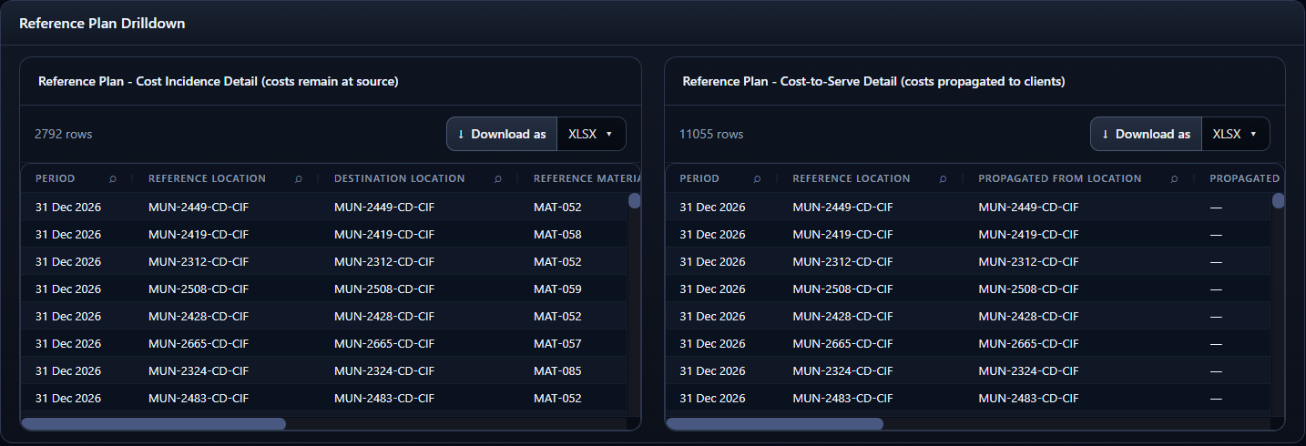
When reconciling the detailed export, count each economic event once:
use records marked triggeringEvent = true and their triggeringEventValue, grouped by P&L line type and the event's reference location.
Do not remove a fixed cost simply because its associated quantity is zero.
Check excluded locations, facilities closed by optimization, and open idle
facilities separately.
Compare the flexible network with brownfield
Now select 19 in Reference Supply Plan and 23 in (Optional) Comparison Supply Plan. Keep the same aggregation and the complete regional-plan scope, then click Submit.
The Cost Incidence Value pivot shows higher internal and delivery freight alongside lower fixed cost. Read the components together before interpreting the total.
Results of the three runs
The table displays costs as positive values in the scenario's monetary unit; the pivot above shows them as negative incidences. Totals were calculated before rounding the individual components.
| Metric | Baseline 18 | Flexible 19 | Brownfield 23 |
|---|---|---|---|
| Demand (TON) | 243,903.353333 | 243,903.353333 | 243,903.353333 |
| Fulfilled (TON) | 238,761.385000 | 241,782.401667 | 241,782.402848 |
| Unfulfilled (TON) | 5,141.968333 | 2,120.951667 | 2,120.950485 |
| Fulfillment (%) | 97.891801 | 99.130413 | 99.130414 |
| Internal freight | 17,272,087.10 | 16,918,514.60 | 17,780,648.16 |
| Delivery freight | 12,116,786.82 | 12,179,209.57 | 13,754,018.70 |
| Location fixed cost | 21,544,289.56 | 21,544,289.56 | 18,767,154.37 |
| Observed logistics total | 50,933,163.49 | 50,642,013.72 | 50,301,821.24 |
| Logistics cost / fulfilled TON | 213.3224 | 209.4529 | 208.0458 |
Brownfield reduces observed logistics cost by 340,192.48, approximately 0.67%, relative to the flexible network. Fulfillment differs by only 0.001181 TON because of CP-SAT numerical precision; both are approximately 99.1304%. The baseline fulfills less demand, so its comparison must also account for the service improvement.
FOB deliveries have real volume in all three plans and zero delivery-freight incidence. Brownfield delivers approximately 80,069.446905 TON FOB. Internal transfers remain costed; FOB did not make DC replenishment free.
Check which facilities were selected
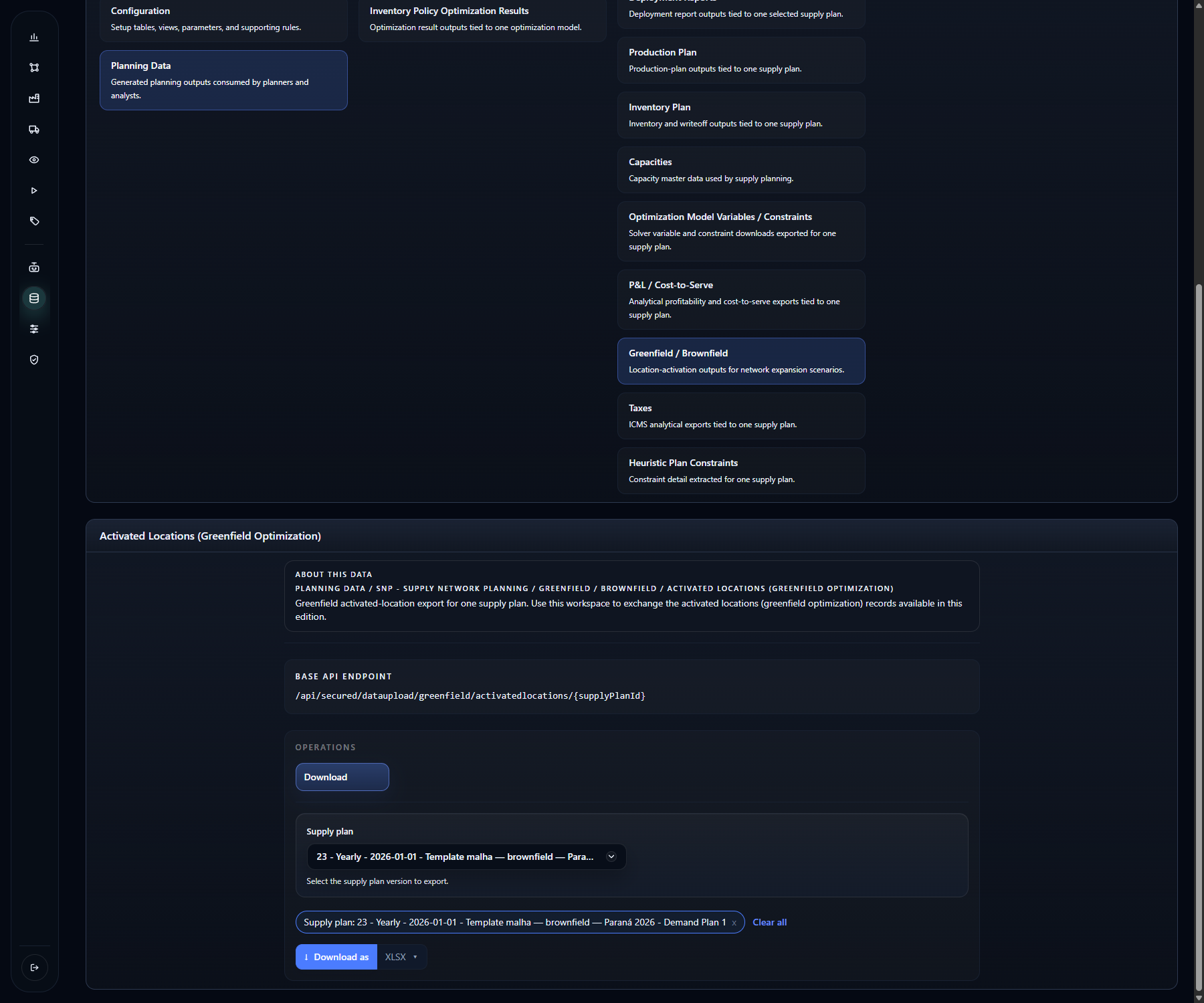
In Data > Data Operations, select Planning Data > SNP - Supply Network
Planning > Greenfield / Brownfield > Activated Locations (Greenfield
Optimization). Choose Supply plan = 23, Download, and Download as
XLSX. Reopen the file and check Location Activated for each optional
facility: 1 means activated and 0 means not activated.
| Optional facilities | Observed decision |
|---|---|
CD-038, CD-039, CD-060, CD-066 |
Activated |
CD-031, CD-062 |
Not activated |
CD-NOVO-001 |
Not activated |
CD-030 and FAB-023 remain fixed in the study. The P&L records fixed cost
at six active facilities, including those two fixed sites. The new
barycenter proposal was not selected: the example demonstrates rationalizing
the existing network without recommending that the candidate open.
Numerical limit of the solution
In this run, the solver reported OPTIMAL, but the recomputed economic
objective was 930,920,479.9522, against a bound of 951,767,613.6384.
The residual gap is approximately 2.2394%, calculated as
(bound − objective) / |objective|. Internal conversion of the decimal
objective requires this qualification: this is an audited feasible solution,
without proof of the exact economic optimum.
The objective reconciles 4,000 × fulfilled TON − freight − fixed costs
of optional facilities. The invariant fixed costs of CD-030 and FAB-023
remain fully included in the P&L even though they do not change the choice
among activation alternatives. Check the objective and report total against
their respective components.
That objective includes the profile's synthetic fulfillment value; it is not revenue or margin, and its gap is not the logistics-cost reduction in the table. Before an investment decision, extend the economic analysis, service target, and solution verification according to the study assumptions.
Export datasets for verification
In Data > Data Operations, select Planning Data > SNP - Supply Network Planning > Fulfilled Demand > Direct Demand for Supply Plan. Choose Download, select Plan period, the Supply plan, and its Plan period = 2026. Keep XLSX and click Download as. The screenshot uses flexible plan 19; repeat for each compared plan.
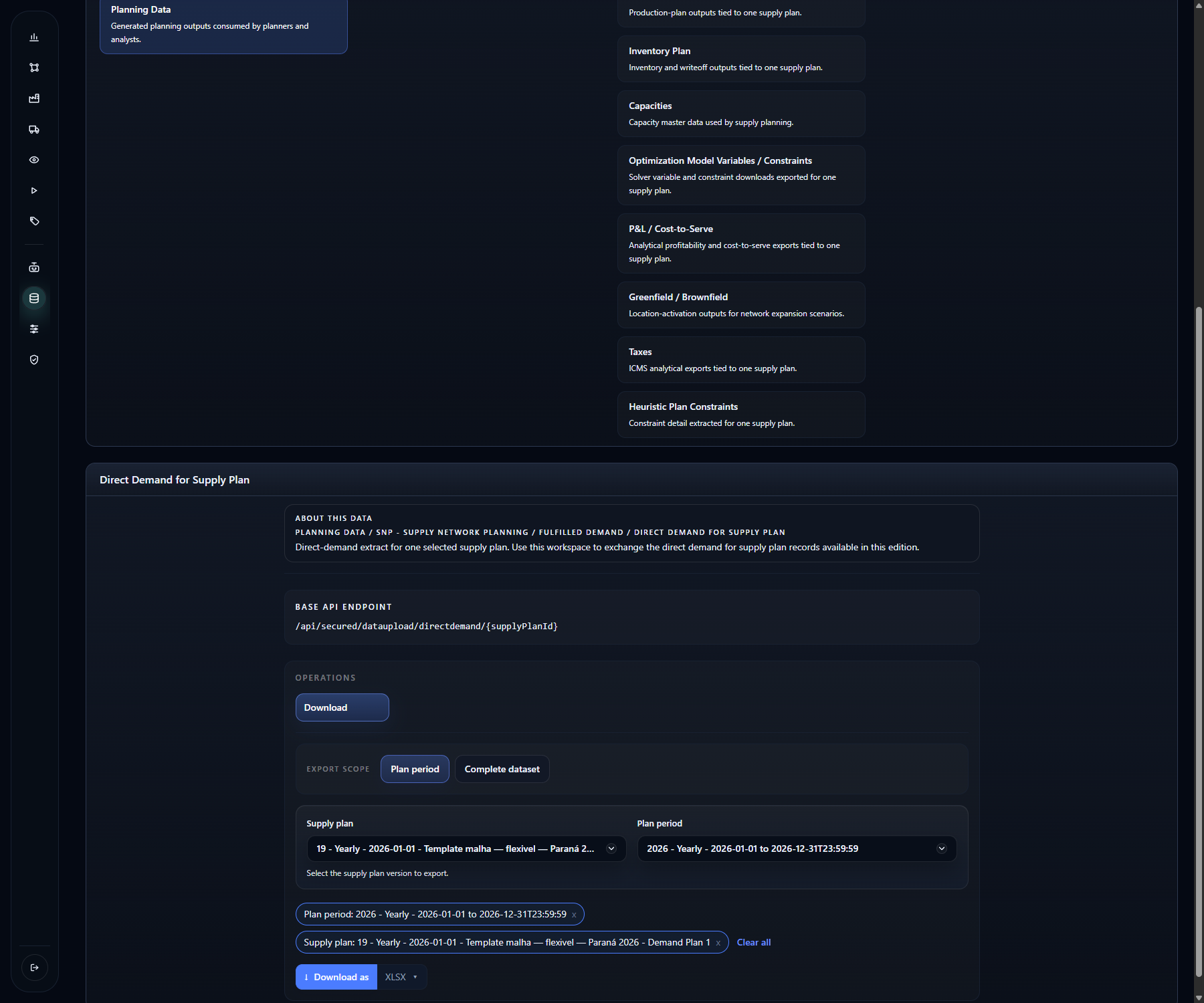
Reopen the workbook and check plan identifier, period, and unit. Compare reference demand, considered demand, and fulfillment for the same client locations. Do not add propagated internal demand as if it were additional market consumption.
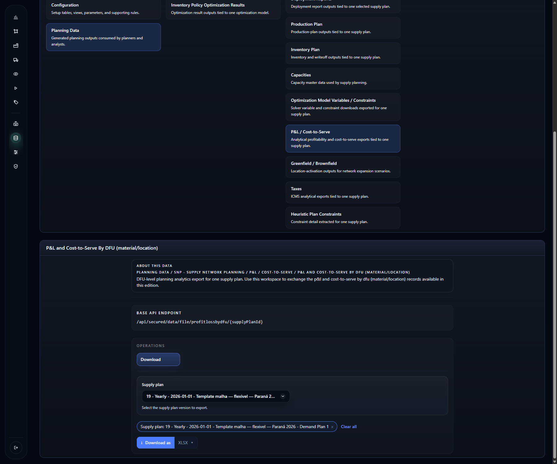
For financial data, use **Planning Data > SNP - Supply Network Planning
P&L / Cost-to-Serve > P&L and Cost-to-Serve By DFU (material/location)**. Select the plan whose financial generation has completed and download it. Reconcile incidence events as described above and retain the files alongside the study assumptions. This training demonstrates the export but does not distribute the scenario's datasets.
Check before continuing
The run completed without error and results were reconciled. The comparison uses the same demand and economic basis, identifies selected facilities, and records assumptions.
Previous: 6. Configure optimization and brownfield profiles.
Next: Training map.