Economic decision data model
Economic planning does not start with a P&L report. It starts with physical decisions—what was sold, produced, purchased, transferred, held, served, or lost—and connects them to the prices, costs, taxes, and policy assumptions that give those decisions economic meaning.
This page is a relationship map. It connects the main data families used by Inventory Optimization and Cost-to-Serve; it is not the upload contract for a single data set.
Where the data appears
- Data → Data Operations contains the master, transactional, configuration, and planning records that feed the calculations.
- Visibility → Inventory Optimization compares candidate inventory policies through service and economic impact.
- Visibility → P&L / Cost-to-Serve reads a saved Supply Plan through revenue, cost, tax, and contribution.
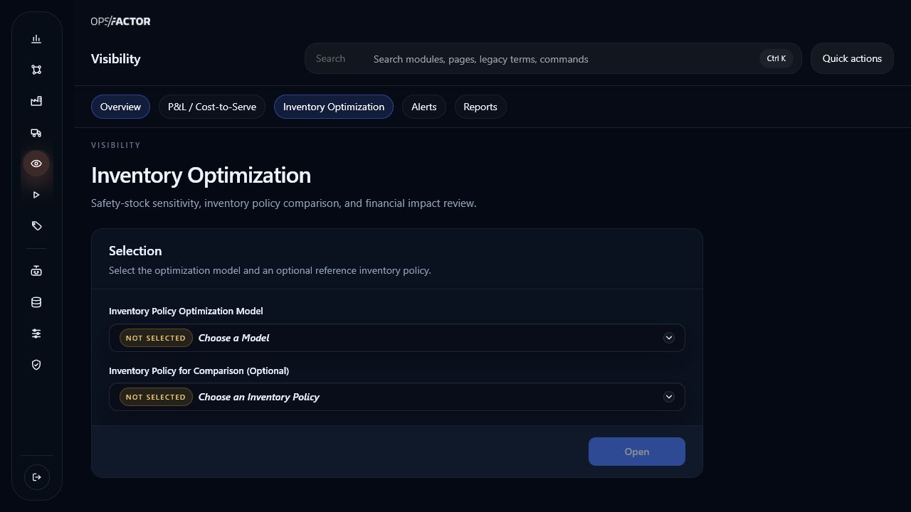
Policy economics
Inventory Optimization changes protection and measures service, stock, stockout, write-off, and economic impact.
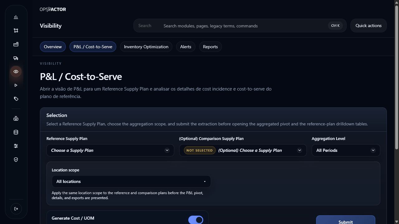
Plan economics
Cost-to-Serve preserves the physical plan and explains how its flows produce revenue, cost, and contribution.
Five connected layers
| Layer | Main data | Role in the decision |
|---|---|---|
| Physical requirement and response | Demand Plan, Supply Plan, planned vehicle trips, served demand, production, purchase, transfer, and inventory | Establishes what the scenario physically required and executed |
| Commercial value | Sell-in, prices, discounts, taxes, and COGS | Values demand and sales at the relevant product, customer or channel, location, and period |
| Operating cost | Material purchase, production costs, and logistics and location costs | Assigns cost to the objects and events that consume resources |
| Policy and uncertainty | Inventory positions, inventory policies, lead time, replenishment reliability, shelf life, and demand variation | Defines the protection candidates and risk simulated by Inventory Optimization |
| Economic evidence | Inventory-policy simulation results, P&L facts, transmitted balances, consolidated lines, and plan comparison | Explains why a policy or physical scenario creates a different economic outcome |
Grains must remain explicit
| Decision object | Logical grain | Why it cannot be flattened early |
|---|---|---|
| Price or COGS | material, optionally customer/channel and location, validity or period, and version | The same material can have different commercial value by market and time |
| Operating cost | cost object, location, resource, routing, lane, vehicle or order, and period | A total cost cannot explain which physical choice generated it |
| Inventory-policy parameter | model, material, location, and applicable validity or scenario | Protection is chosen for an item-location under one loaded set of assumptions |
| Inventory simulation | model, material, location, candidate policy, sample, and period | Average impact depends on the simulated curve and its stochastic samples |
| P&L fact | Supply Plan, economic line type, period, material and location; optionally origin, destination, resource, or bill of material | The economic event must remain traceable to its physical origin |
| Transmitted balance | original economic fact plus the reference material-location-period and propagation direction | Cost-to-Serve must preserve how value moved through transfers, production, inventory, and sales |
Main relationships
| Origin | Relationship | Destination |
|---|---|---|
| Demand Plan | creates the future requirement evaluated by | the Supply Plan and policy simulations |
| Supply Plan | persists physical facts consumed by | Cost-to-Serve and scenario comparison |
| Consolidated planned loading orders | multiply cost per trip by planned trips and allocate it to | distributed materials on the same lane and period |
| Sell-in, prices, and COGS | value | served demand and customer-product-market outcomes |
| Production costs and logistics and location costs | value | the resource, route, inventory, or node that generated the expense |
| Inventory positions and inventory policies | initialize and constrain | candidate-policy simulation |
| Inventory Optimization | produces | service, stock, stockout, write-off, and economic impact by candidate |
| A physical or commercial event | creates | an original P&L fact |
| Transfers, production, inventory, and sales | propagate or allocate | the economic fact through the operating network |
| Detailed economic facts | consolidate into | P&L, contribution, Cost-to-Serve, and plan-comparison views |
Two analyses, one economic vocabulary
Inventory Optimization and Cost-to-Serve use related concepts but answer different questions:
- Inventory Optimization changes a candidate policy and simulates its consequences. Its comparison needs explicit capital, write-off, and shortage economics for the loaded model.
- Cost-to-Serve keeps the saved physical plan and traces economic facts through the network. It explains where revenue, COGS, production, logistics, storage, and other costs were generated or transmitted.
Do not assume that one calculation automatically supplied every economic input to the other. Confirm the economic source and version loaded for each run.
Data-quality checklist
- Confirm the Demand Plan and Supply Plan versions and their common horizon.
- Confirm the default planning UOM and every required conversion.
- Verify price, COGS, tax, and cost validity for the scenario period.
- Separate missing data from a true zero value.
- Check that lanes, resources, routings, vehicles, and locations referenced by a cost are part of the selected scenario.
- Verify whether stockout becomes lost sales, backlog, substitution, or another economic consequence.
- Confirm shelf life, aging, and write-off behavior before comparing coverage.
- Trace a surprising consolidated number back to its physical event and original economic fact.
Continue
- Review the functional policy journey in Inventory policies and optimization.
- Review physical-plan economics in Cost-to-Serve and P&L.
- Configure commercial value in Prices and material cost in COGS.
- Configure manufacturing valuation in Production costs.
- Configure network, storage, handling, transfer, and tax valuation in Logistics and location costs.
- Follow all physical dependencies in the Supply Planning data model.
- See the economic trade-off in the inventory-policy article.
- Organize the process evolution in the inventory policy maturity article.
- See demand, network, cost, and margin connected in the industrial network case.
Interpretation boundary
A zero line is not proof of zero cost, and a recommended policy is not an unconditional optimum. Both results depend on the physical plan, loaded versions, units, filters, and economic assumptions.