18. Analyze the Supply Plan results
A completed execution is the starting point for reviewing the plan. This chapter uses the Supply Plan created in chapter 16 to answer four questions: what must be produced, where capacity is consumed, how material reaches its destination, and how much inventory remains.
1. Select one scenario for the entire review
Open Supply Chain Planning > Supply Plans and find the description used in
chapter 16. Check the reference period, execution profile, supply network and
reference Demand Plan. Record the plan ID (Supply Plan Id): every extract and Planning Book
selection in this review must use that same ID.
The tutorial starts on January 1, 2027, uses TON as its common Supply
Planning unit and considers the initial stock loaded in chapter 14. An ID is
assigned by each installation; a different numeric ID is not a discrepancy.
The documented execution uses Supply Plan 6, Demand Plan 1, profile
PA_TUTORIAL_PRIORIDADE_LOCAL_2027 and network MALHA_PADRAO_V2. The screenshots
and five files below belong to this calculation, with no subsequent Working Plan
adjustments.
These results were collected on Community 2026.09.22, after the production-plan persistence and constrained-plan physical-reconciliation fixes. In another installation, check the version, profile, calendar, data and IDs before comparing values; repeat the extracts and balance checks for your own plan.
Keep the three series separate:
| Series | How to interpret it |
|---|---|
| Unconstrained Plan | Complete requirement before final feasibility cuts. The Community heuristic may level production across origins and periods while retaining the residual it could not allocate. |
| Constrained Plan | Result after the active restrictions have been applied. It may fulfill less than the complete requirement. |
| Working Plan | Operational series selected by the execution profile; manual changes may make it differ from the original calculated result. |
Completed confirms the end of execution. It does not prove full demand fulfillment, feasibility of every unconstrained line or a global cost optimum. Community uses a sequential heuristic.
2. Open Production Overview
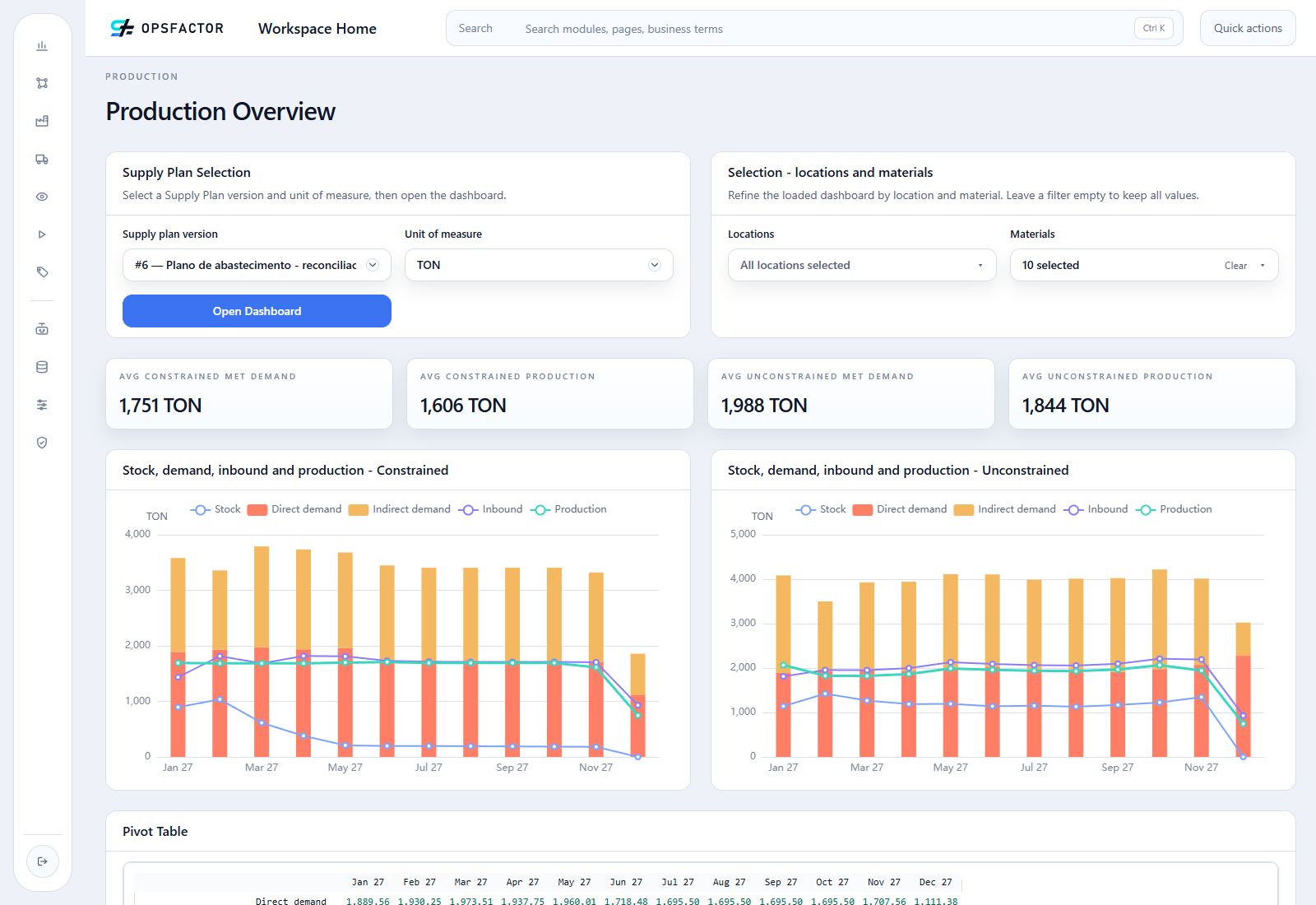
Open Production > Production Overview. In Supply Plan Selection, choose
the same Supply plan version, set Unit of measure to TON and click
Open Dashboard. Locations and Materials are independent optional
multiselects: an empty selection includes every value in that scope. Select
finished goods to avoid combining manufacturing stages; select one plant when
investigating its local result.
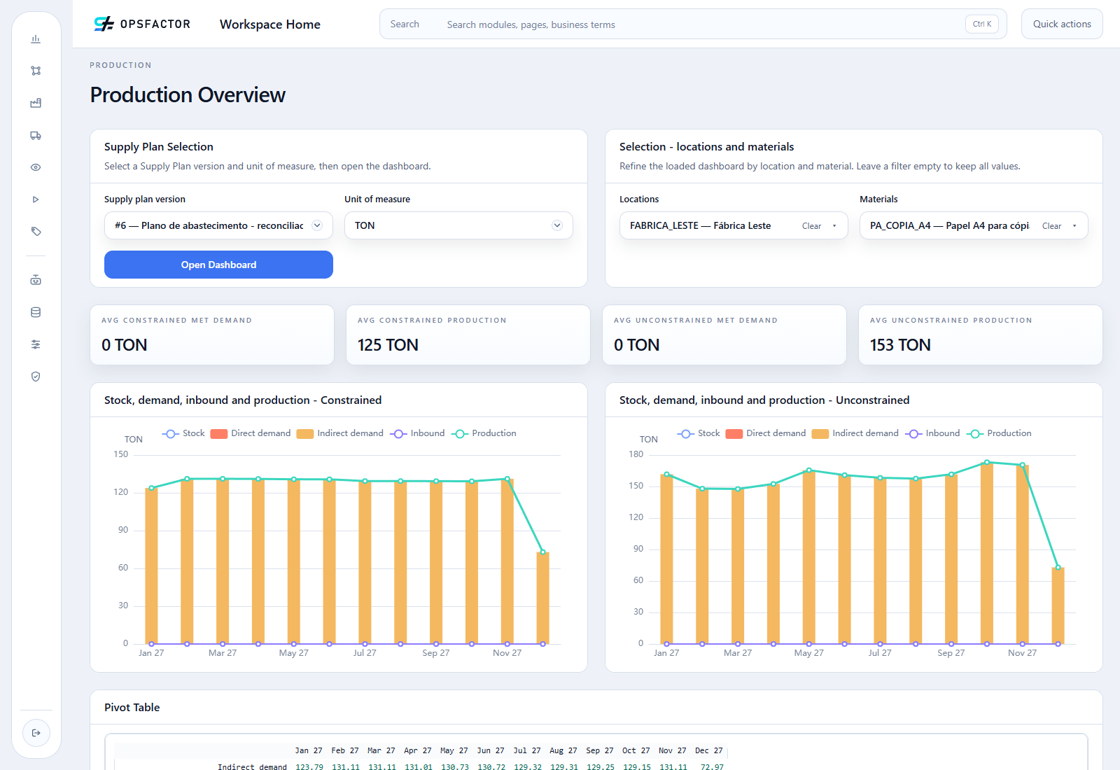
Read Stock, demand, inbound and production - Constrained alongside the Unconstrained chart, using the same materials, locations and periods. Compare production, inbound and stock separately from direct and indirect demand. Cards labeled Avg are averages per period, not horizon totals.
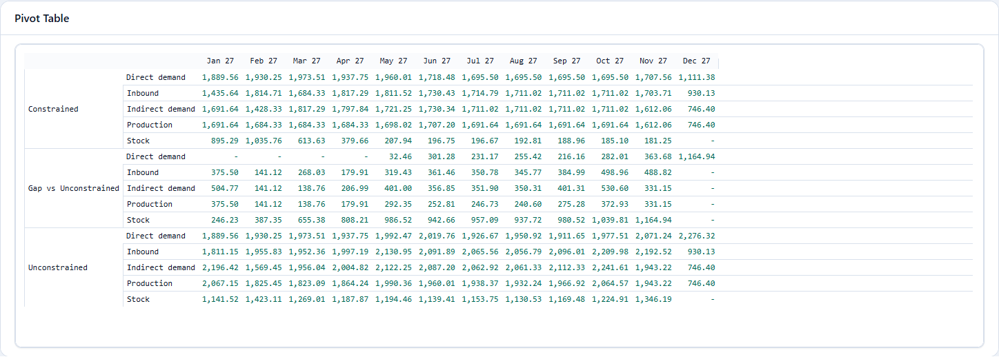
The Pivot Table keeps planVersion, series and period separate and
includes Gap vs Unconstrained. A gap is unconstrained minus constrained
for that series. It becomes a service conclusion only after examining the
direct-demand result at the demand locations; a production gap at a plant
is not interchangeable with unmet demand at a customer.
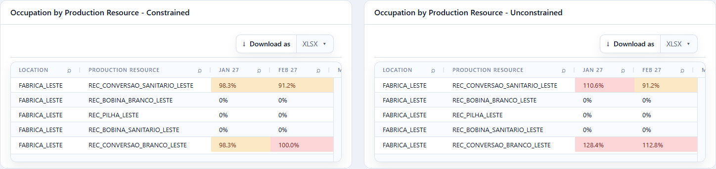
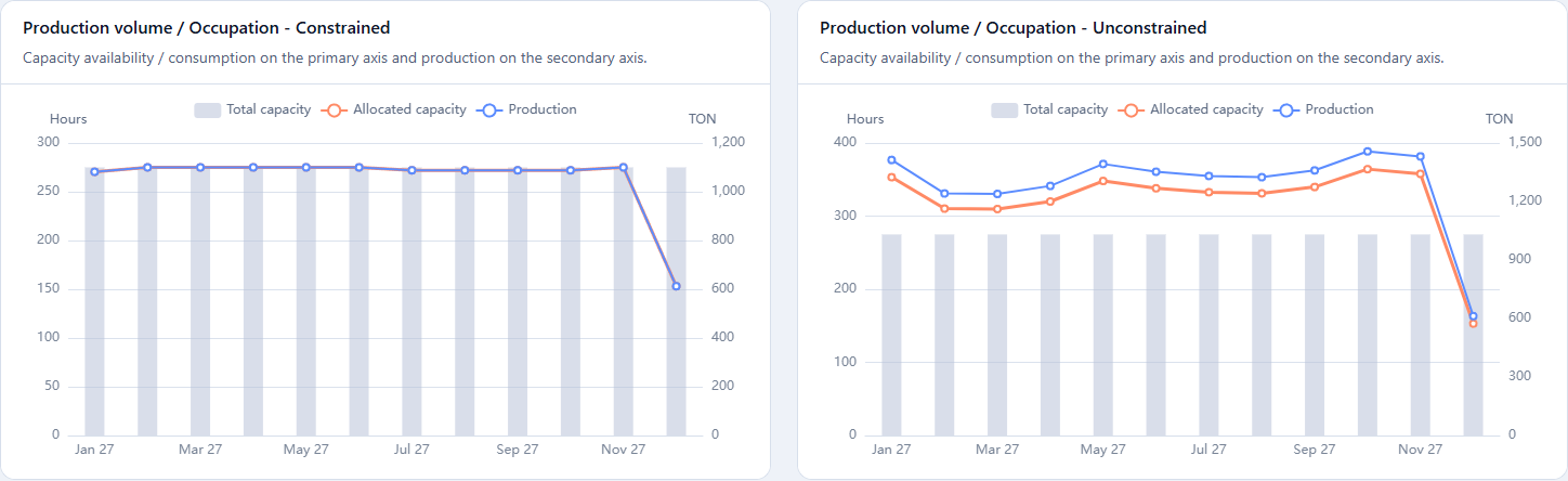
Below the pivot, use Production resources to narrow the occupation charts and both Occupation by Production Resource grids. The charts compare capacity availability and consumption on the primary axis and production on the secondary axis. Do not compare the height of quantities on different axes as if they used the same unit.
The occupation heatmap has one resource per row and one period per column.
Compare the same cell in Constrained and Unconstrained. A percentage
uses consumed capacity divided by available capacity; — means a valid
percentage is unavailable. The visual alerts start above 80% and become stronger
from 99.9%; a colored cell alone does not prove demand loss or its cause.
Click a period cell to open Production Resource Detail below the grids. Confirm Production line, Location, Period and available capacity. Inspect Material, Production version, Routing, BOM, UOM and Capacity UOM, then compare these columns:
| Detail label | Plan series |
|---|---|
| Unrestricted qty / Unrestricted consumption | Unconstrained |
| Restricted qty / Restricted consumption | Constrained |
| Work plan qty / Work plan consumption | Working |
The detail retains the production and capacity units returned for that
resource. It is not necessarily converted to the dashboard's selected TON.
Preserve those units when reconciling it with the original exports. This is a
read-only drilldown; selecting a different filter or scenario clears the old
detail so it cannot be mistaken for the new selection.
3. Download the five detailed results
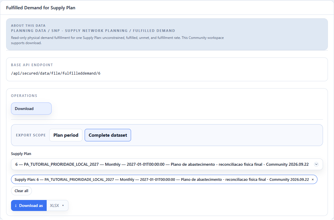
Open Data > Operations > Data Operations, select Planning Data and SNP - Supply Network Planning. For each topic below, select Supply Plan 6, XLSX and Download as. For Fulfilled Demand for Supply Plan, also select Complete dataset to include all periods. The other four topics export the selected plan without this scope selector.
| Result / screen topic | Original download | Rows |
|---|---|---|
| Fulfilled Demand > Fulfilled Demand for Supply Plan | Fulfilled demand | 720 |
| Production Plan > Production Plan - Volumes | Production volumes | 391 |
| Production Plan > Production Plan - Resource Occupation | Resource occupation | 391 |
| Purchase/Distribution Plan > Purchase/Distribution Plan | Distribution | 1061 |
| Inventory Plan > Inventory Plan | Projected inventory | 278 |
Download all five originals as ZIP.
Preserve the original download
Preserve the exported XLSX bytes: headers, sheets, order, values, types and native formatting. Do not translate or decorate the workbook. Use a separate copy for formulas and analysis. The previews only read the originals.
The inventory result includes the December 31, 2026 opening balance and the planning horizon; do not remove that row from the original file. Row counts identify the extraction but do not establish balance or feasibility.
Fulfilled demand
Literal preview of the first 5 rows; sheet Data, 720 data rows.
| Supply Plan Id | Location Id | Location Description | Material Id | Material Description | Reference Date | Unit of Measure Id | Unconstrained Demand | Fulfilled Demand | Unmet Demand | Fulfillment Rate |
|---|---|---|---|---|---|---|---|---|---|---|
| 6 | REGIONAL_CENTRO_DIRETO | Regional Centro — canal direto | PA_BRANCO_75_A4_100 | Papel branco A4 75 g/m² — 100 folhas | 2027-01-31T23:59:59 | TON | 9.641457211332794 | 9.641457211332794 | 0 | 1 |
| 6 | REGIONAL_CENTRO_DIRETO | Regional Centro — canal direto | PA_BRANCO_75_A4_100 | Papel branco A4 75 g/m² — 100 folhas | 2027-02-28T23:59:59 | TON | 9.903106503861773 | 9.903106503861773 | 0 | 1 |
| 6 | REGIONAL_CENTRO_DIRETO | Regional Centro — canal direto | PA_BRANCO_75_A4_100 | Papel branco A4 75 g/m² — 100 folhas | 2027-03-31T23:59:59 | TON | 10.197754641973477 | 10.197754641973477 | 0 | 1 |
| 6 | REGIONAL_CENTRO_DIRETO | Regional Centro — canal direto | PA_BRANCO_75_A4_100 | Papel branco A4 75 g/m² — 100 folhas | 2027-04-30T23:59:59 | TON | 9.96174099706871 | 9.96174099706871 | 0 | 1 |
| 6 | REGIONAL_CENTRO_DIRETO | Regional Centro — canal direto | PA_BRANCO_75_A4_100 | Papel branco A4 75 g/m² — 100 folhas | 2027-05-31T23:59:59 | TON | 10.317966386863628 | 10.317966386863628 | 0 | 1 |
Production volumes
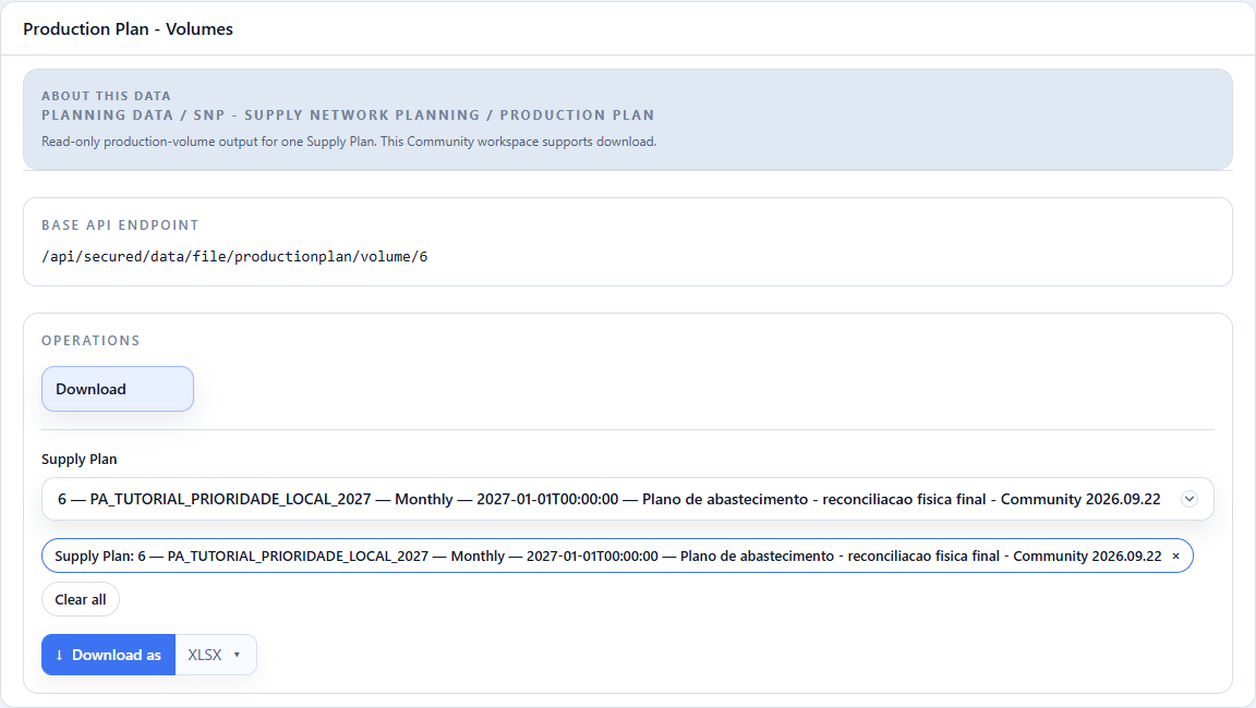
Literal preview of the first 5 rows; sheet Data, 391 data rows.
| Supply Plan Id | Location Id | Output Material Id | Planned Date | Production Version Id | Routing Id | Bill of Materials | Unit of Measure Id | Unconstrained Planned Order Quantity | Unconstrained Firm Order Quantity | Constrained Planned Order Quantity | Constrained Firm Order Quantity | Default SNP Unit of Measure | Unconstrained Total Planned Order Quantity in default SNP unit | Unconstrained Total Firm Order Quantity in default SNP unit | Constrained Total Planned Order Quantity in default SNP unit | Constrained Total Firm Order Quantity in default SNP unit |
|---|---|---|---|---|---|---|---|---|---|---|---|---|---|---|---|---|
| 6 | FABRICA_LESTE | BOBINA_BRANCO_75 | 2027-01-31T23:59:59 | VP_TUTORIAL_001 | ROTEIRO_FABRICA_LESTE_BOBINA_BRANCO_75 | LT_FABRICA_LESTE_BOBINA_BRANCO_75 | TON | 931.1901773235801 | 0 | 712.5332287874572 | 0 | TON | 931.1901773235801 | 0 | 712.5332287874572 | 0 |
| 6 | FABRICA_LESTE | BOBINA_BRANCO_75 | 2027-02-28T23:59:59 | VP_TUTORIAL_001 | ROTEIRO_FABRICA_LESTE_BOBINA_BRANCO_75 | LT_FABRICA_LESTE_BOBINA_BRANCO_75 | TON | 814.3832591321747 | 0 | 725.4143960243055 | 0 | TON | 814.3832591321747 | 0 | 725.4143960243055 | 0 |
| 6 | FABRICA_LESTE | BOBINA_BRANCO_75 | 2027-03-31T23:59:59 | VP_TUTORIAL_001 | ROTEIRO_FABRICA_LESTE_BOBINA_BRANCO_75 | LT_FABRICA_LESTE_BOBINA_BRANCO_75 | TON | 812.8333573144084 | 0 | 725.4143960243056 | 0 | TON | 812.8333573144084 | 0 | 725.4143960243056 | 0 |
| 6 | FABRICA_LESTE | BOBINA_BRANCO_75 | 2027-04-30T23:59:59 | VP_TUTORIAL_001 | ROTEIRO_FABRICA_LESTE_BOBINA_BRANCO_75 | LT_FABRICA_LESTE_BOBINA_BRANCO_75 | TON | 839.5364624451364 | 0 | 725.1374783622155 | 0 | TON | 839.5364624451364 | 0 | 725.1374783622155 | 0 |
| 6 | FABRICA_LESTE | BOBINA_BRANCO_75 | 2027-05-31T23:59:59 | VP_TUTORIAL_001 | ROTEIRO_FABRICA_LESTE_BOBINA_BRANCO_75 | LT_FABRICA_LESTE_BOBINA_BRANCO_75 | TON | 912.4184230753658 | 0 | 717.404682066702 | 0 | TON | 912.4184230753658 | 0 | 717.404682066702 | 0 |
Resource occupation
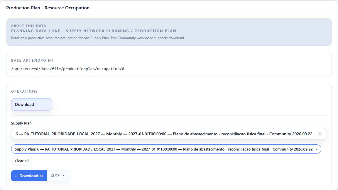
Literal preview of the first 5 rows; sheet Data, 391 data rows.
| Supply Plan Id | Location Id | Output Material Id | Planned Date | Production Version Id | Routing Id | Bill of Materials | Resource Id | Routing Cluster | Resource Capacity Unit of Measure | Resource Capacity Period | Unit of Measure Id | Unconstrained Planned Order Quantity | Unconstrained Firm Order Quantity | Unconstrained Total Resource Consumption | Constrained Planned Order Quantity | Constrained Firm Order Quantity | Constrained Total Resource Consumption | Default SNP Unit of Measure | Unconstrained Planned Order Quantity in default SNP unit | Unconstrained Firm Order Quantity in default SNP unit | Constrained Planned Order Quantity in default SNP unit | Constrained Firm Order Quantity in default SNP unit | Set-up time (hours) | Set-up sequence for current period |
|---|---|---|---|---|---|---|---|---|---|---|---|---|---|---|---|---|---|---|---|---|---|---|---|---|
| 6 | FABRICA_LESTE | BOBINA_BRANCO_75 | 2027-01-31T23:59:59 | VP_TUTORIAL_001 | ROTEIRO_FABRICA_LESTE_BOBINA_BRANCO_75 | LT_FABRICA_LESTE_BOBINA_BRANCO_75 | REC_BOBINA_BRANCO_LESTE | Hours | 280 | TON | 931.1901773235801 | 0 | 223.4856425576592 | 712.5332287874572 | 0 | 171.00797490898972 | TON | 931.1901773235801 | 0 | 712.5332287874572 | 0 | |||
| 6 | FABRICA_LESTE | BOBINA_BRANCO_75 | 2027-02-28T23:59:59 | VP_TUTORIAL_001 | ROTEIRO_FABRICA_LESTE_BOBINA_BRANCO_75 | LT_FABRICA_LESTE_BOBINA_BRANCO_75 | REC_BOBINA_BRANCO_LESTE | Hours | 280 | TON | 814.3832591321747 | 0 | 195.45198219172192 | 725.4143960243055 | 0 | 174.0994550458333 | TON | 814.3832591321747 | 0 | 725.4143960243055 | 0 | |||
| 6 | FABRICA_LESTE | BOBINA_BRANCO_75 | 2027-03-31T23:59:59 | VP_TUTORIAL_001 | ROTEIRO_FABRICA_LESTE_BOBINA_BRANCO_75 | LT_FABRICA_LESTE_BOBINA_BRANCO_75 | REC_BOBINA_BRANCO_LESTE | Hours | 280 | TON | 812.8333573144084 | 0 | 195.08000575545802 | 725.4143960243056 | 0 | 174.09945504583334 | TON | 812.8333573144084 | 0 | 725.4143960243056 | 0 | |||
| 6 | FABRICA_LESTE | BOBINA_BRANCO_75 | 2027-04-30T23:59:59 | VP_TUTORIAL_001 | ROTEIRO_FABRICA_LESTE_BOBINA_BRANCO_75 | LT_FABRICA_LESTE_BOBINA_BRANCO_75 | REC_BOBINA_BRANCO_LESTE | Hours | 280 | TON | 839.5364624451364 | 0 | 201.4887509868327 | 725.1374783622155 | 0 | 174.0329948069317 | TON | 839.5364624451364 | 0 | 725.1374783622155 | 0 | |||
| 6 | FABRICA_LESTE | BOBINA_BRANCO_75 | 2027-05-31T23:59:59 | VP_TUTORIAL_001 | ROTEIRO_FABRICA_LESTE_BOBINA_BRANCO_75 | LT_FABRICA_LESTE_BOBINA_BRANCO_75 | REC_BOBINA_BRANCO_LESTE | Hours | 280 | TON | 912.4184230753658 | 0 | 218.9804215380878 | 717.404682066702 | 0 | 172.17712369600847 | TON | 912.4184230753658 | 0 | 717.404682066702 | 0 |
Distribution
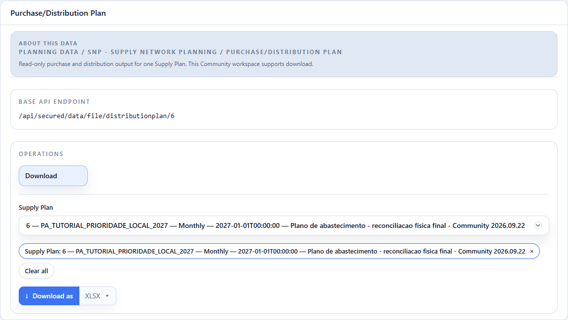
Literal preview of the first 5 rows; sheet Data, 1061 data rows.
| Origin Location Id | Destination Location Id | Product Id | Planned Delivery Date (represents the end of each period : month/week/day) | Suggested Order Emission Date | Unit of Measure Id | Unconstrained Planned Order Quantity | Unconstrained Firm Order Quantity | Constrained Planned Order Quantity | Constrained Firm Order Quantity |
|---|---|---|---|---|---|---|---|---|---|
| CD_INTERIOR | REGIONAL_CENTRO_DIRETO | PA_BRANCO_75_A4_100 | 2027-01-31T23:59:59 | 2027-01-01T00:00:00 | TON | 9.641457211332794 | 0 | 9.641457211332794 | 0 |
| CD_INTERIOR | REGIONAL_CENTRO_DIRETO | PA_BRANCO_75_A4_100 | 2027-02-28T23:59:59 | 2027-02-01T00:00:00 | TON | 9.903106503861773 | 0 | 9.903106503861773 | 0 |
| CD_INTERIOR | REGIONAL_CENTRO_DIRETO | PA_BRANCO_75_A4_100 | 2027-03-31T23:59:59 | 2027-03-01T00:00:00 | TON | 10.197754641973477 | 0 | 10.197754641973477 | 0 |
| CD_INTERIOR | REGIONAL_CENTRO_DIRETO | PA_BRANCO_75_A4_100 | 2027-04-30T23:59:59 | 2027-04-01T00:00:00 | TON | 9.96174099706871 | 0 | 9.96174099706871 | 0 |
| CD_INTERIOR | REGIONAL_CENTRO_DIRETO | PA_BRANCO_75_A4_100 | 2027-05-31T23:59:59 | 2027-05-01T00:00:00 | TON | 10.317966386863628 | 0 | 10.317966386863628 | 0 |
Projected inventory
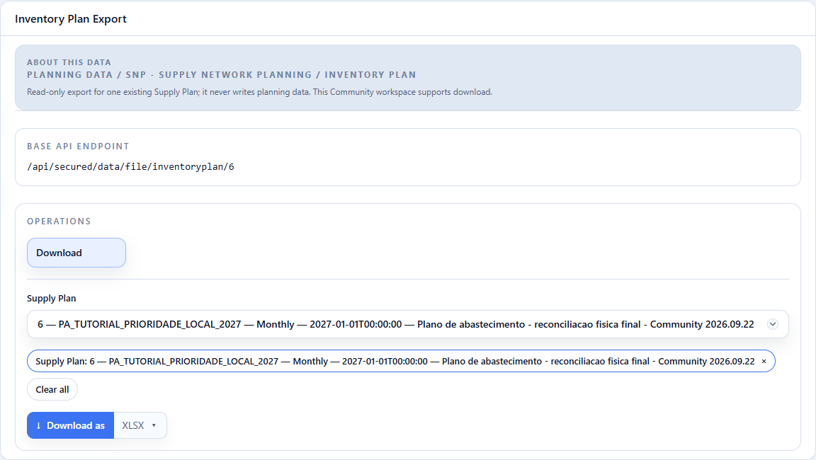
Literal preview of the first 5 rows; sheet Data, 278 data rows.
| Location Id | Product Id | Reference Date (represents the end of each period : month/week/day) | UOM - Unit of Measure Id | Safety Stock Quantity | Maximum Stock Quantity | Projected Stock - Working Version | Projected Stock - Unconstrained Version | Projected Stock - Constrained Version | Default SNP UOM | Projected Stock in SNP UOM - Working Version | Projected Stock in SNP UOM - Unconstrained Version | Projected Stock in SNP UOM - Constrained Version |
|---|---|---|---|---|---|---|---|---|---|---|---|---|
| CD_INTERIOR | PA_BRANCO_75_A4_100 | 2026-12-31T23:59:59 | TON | 0 | 0 | 25.715999603271484 | 25.715999603271484 | 25.715999603271484 | TON | 25.715999603271484 | 25.715999603271484 | 25.715999603271484 |
| CD_INTERIOR | PA_BRANCO_75_A4_100 | 2027-01-31T23:59:59 | TON | 6.1079206642322585 | 21.988514391236134 | 16.249373788976428 | 21.988514391236137 | 16.249373788976428 | TON | 16.249373788976428 | 21.988514391236137 | 16.249373788976428 |
| CD_INTERIOR | PA_BRANCO_75_A4_100 | 2027-02-28T23:59:59 | TON | 6.289650250877443 | 22.6427409031588 | 16.903600300899086 | 22.642740903158796 | 16.903600300899086 | TON | 16.903600300899086 | 22.642740903158796 | 16.903600300899086 |
| CD_INTERIOR | PA_BRANCO_75_A4_100 | 2027-03-31T23:59:59 | TON | 6.144084552054303 | 22.118704387395496 | 3.2946670323910077 | 22.118704387395496 | 3.2946670323910077 | TON | 3.2946670323910077 | 22.118704387395496 | 3.2946670323910077 |
| CD_INTERIOR | PA_BRANCO_75_A4_100 | 2027-04-30T23:59:59 | TON | 6.363793026218862 | 22.909654894387906 | 4.085617539383417 | 22.909654894387906 | 4.085617539383417 | TON | 4.085617539383417 | 22.909654894387906 | 4.085617539383417 |
4. Quantify the production gap
In the volume extract, first select finished goods and the 2027 horizon. Use material characteristics from chapter 2 to identify the production stage. Keep rolls, skids and raw materials in separate analyses: adding their volumes to finished goods counts multiple manufacturing stages of the same flow.
Group the selected rows by Location Id, Output Material Id and Planned Date.
Retain Production Version Id, Routing Id and Bill of Materials when
investigating which alternative was selected. Use either the native quantity
columns or the columns converted to the default SNP unit, consistently.
For the converted quantities, calculate:
- unconstrained production =
Unconstrained Total Planned Order Quantity in default SNP unit+Unconstrained Total Firm Order Quantity in default SNP unit; - constrained production =
Constrained Total Planned Order Quantity in default SNP unit+Constrained Total Firm Order Quantity in default SNP unit; - production gap = unconstrained production − constrained production.
The recorded tutorial result provides this finished-goods comparison:
| Measure | TON |
|---|---|
| Unconstrained production | 22,122.030 |
| Constrained production | 19,274.900 |
| Difference, using the displayed rounded totals | 2,847.130 |
This is a production reduction, not a direct measure of lost sales or unfulfilled customer demand. Initial stock, transfer timing, inventory targets and intermediate production can change the relationship between production and customer service. Keep full precision in the analysis and round only for presentation.
Locate the difference
Start with the finished-goods total, then break it down by plant, material and month. Choose one nonzero gap and retain its complete key for the capacity and material-flow checks below. Also look for production shifted to an earlier month or another plant; a local reduction may be offset elsewhere in the horizon.
5. Check occupation against availability
In the occupation extract, use Resource Id and Planned Date to sum
Unconstrained Total Resource Consumption and
Constrained Total Resource Consumption separately. Compare each total with
the availability of the same resource and period loaded in
chapter 11. Check Resource Capacity Unit of Measure
and Resource Capacity Period before comparing values.
| Observation | Next check |
|---|---|
| Unconstrained consumption exceeds availability | Identify competing materials and production versions on that resource and month. |
| Constrained production falls while this resource has spare capacity | Follow its components, eligible alternatives, lead times and other resources; spare capacity at one operation does not establish feasibility of the chain. |
| An earlier month or another plant absorbs production | Check the changed production version, component requirements and transfer dates before interpreting the reallocation. |
| Several operations consume resources for the same production row | Sum consumption by resource; do not sum repeated production quantities across operations. |
Where availability is positive, utilization is consumption divided by available capacity in the same unit and period. Zero availability with positive consumption is an exception to investigate, not 0% utilization. Do not infer a complete causal explanation from the production difference alone.
Example: white-paper converting in October
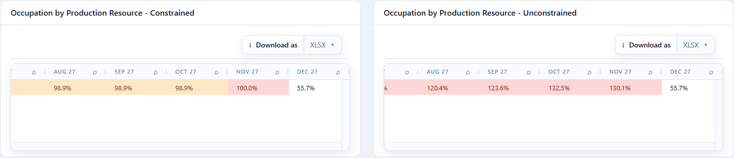
Filter Production resources to REC_CONVERSAO_BRANCO_LESTE at
FABRICA_LESTE. In October 2027 the Unconstrained grid shows 132.5%:
364.253085 h against 275 h available. The matching Constrained cell
shows 98.9%, approximately 271.984369 h. Click the cell above 100% to inspect
the eight products competing for that line.

Open original-size screenshot
For PA_BRANCO_75_A4_100, inspect version VP_TUTORIAL_004, routing
ROTEIRO_FABRICA_LESTE_PA_BRANCO_75_A4_100 and BOM
LT_FABRICA_LESTE_PA_BRANCO_75_A4_100. Production is in TON; consumption is
in Hours. At 4 TON/h, 187.329044 TON / 4 = 46.832261 h unconstrained
and 139.657622 TON / 4 = 34.914405 h constrained. Working Plan equals the
constrained result in this execution. Sum the eight rows of hours to reconcile
the cell; one product does not represent the whole line. Open the full image
to read all columns.

6. Follow distribution to the destination
Select the material under investigation in the distribution result. Review origin, destination, period, quantity and unit. Follow the supply chain from the plant through the DC to the demand location, using the network configured in chapter 12.
Check that each flow has an eligible lane and material, and that its lead time allows arrival when required. Compare constrained and unconstrained flows within the same scenario and time convention. A transfer leaving an origin and the corresponding receipt at its destination are two views of one flow. Summing every leg of a multi-stage network does not measure final demand.
7. Reconcile inventory and demand
At each selected material-location, start from the stock at the beginning of January 1, 2027. Follow production, receipts and consumption through the planning buckets, checking whether the output uses opening or closing stock. Use dispatch dates at origins and receipt dates at destinations; a lead time may place the two events in different buckets.
The reconciliation is opening stock plus inflows minus outflows equals closing stock, with the movements actually present in the selected scenario. Compare closing stock with the inventory target from chapter 13. A 5-day policy is a target rule; it does not guarantee 5 days of stock after capacity and supply restrictions.
In the Supply Planning Book, select the same plan, a configured view and the planning location. A configured view for the current user is required. Inspect the Community Working Plan measures:
| Measure | Review purpose |
|---|---|
| Total Demand, Direct Demand, Direct Demand - Demand Plan | Distinguish the total requirement from its direct-demand components. Do not add a total to its components. |
| Indirect Demand | Identify requirements propagated from downstream production or distribution. |
| Safety Stock | Inspect the target used for this material-location-period. |
| Stock | Follow the projected inventory position. |
| Planned Production, Planned Inbound | Connect local production and receipts to the inventory position. |
These Community Planning Book measures belong to Working Plan. Use the detailed extracts for the unconstrained-versus-constrained comparison. If the Working Plan was manually changed, reconcile those changes separately before comparing it with the execution baseline. This review does not require editing cells or saving a new operational plan.
Configure a finished and semi-finished goods view
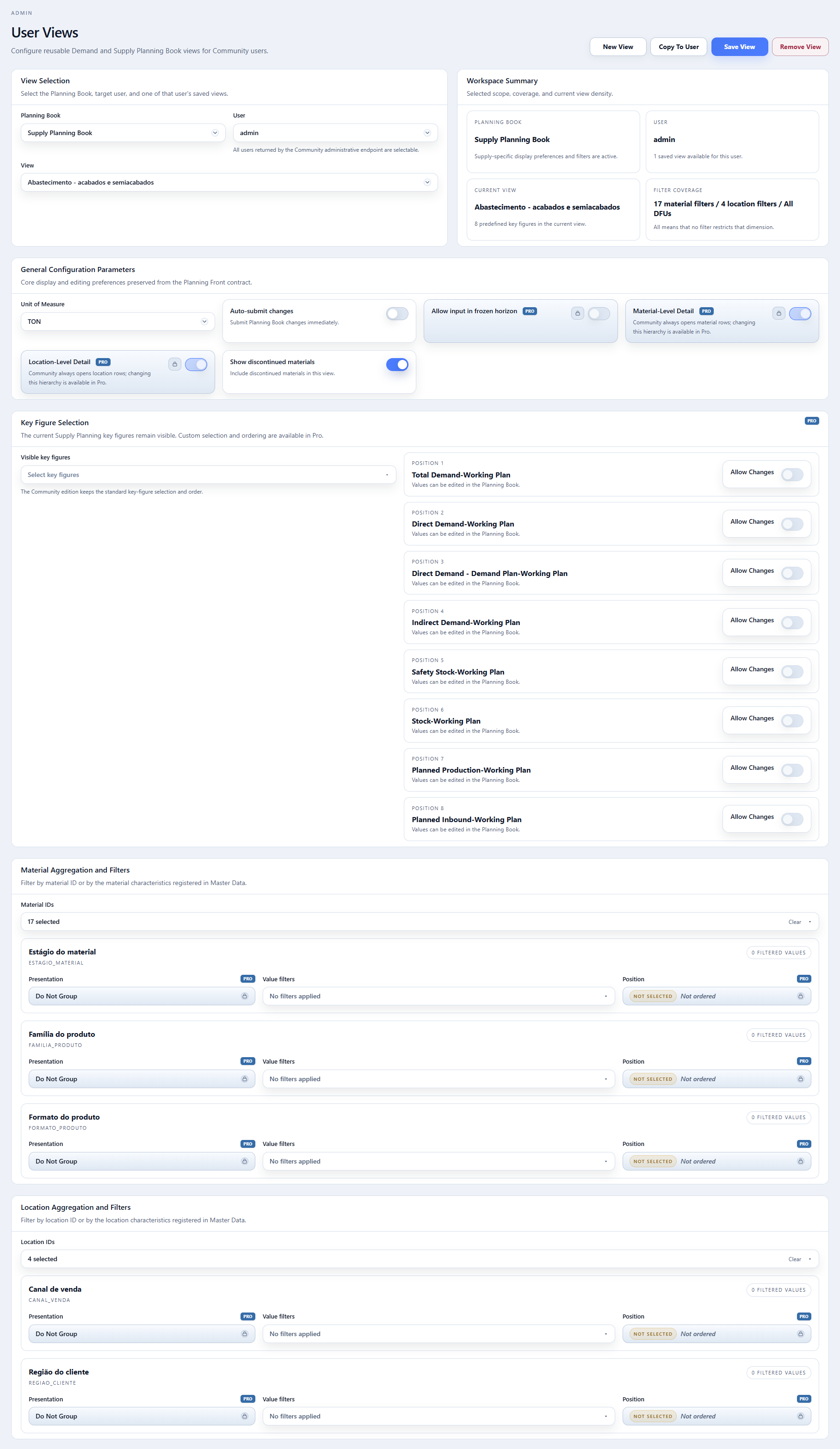
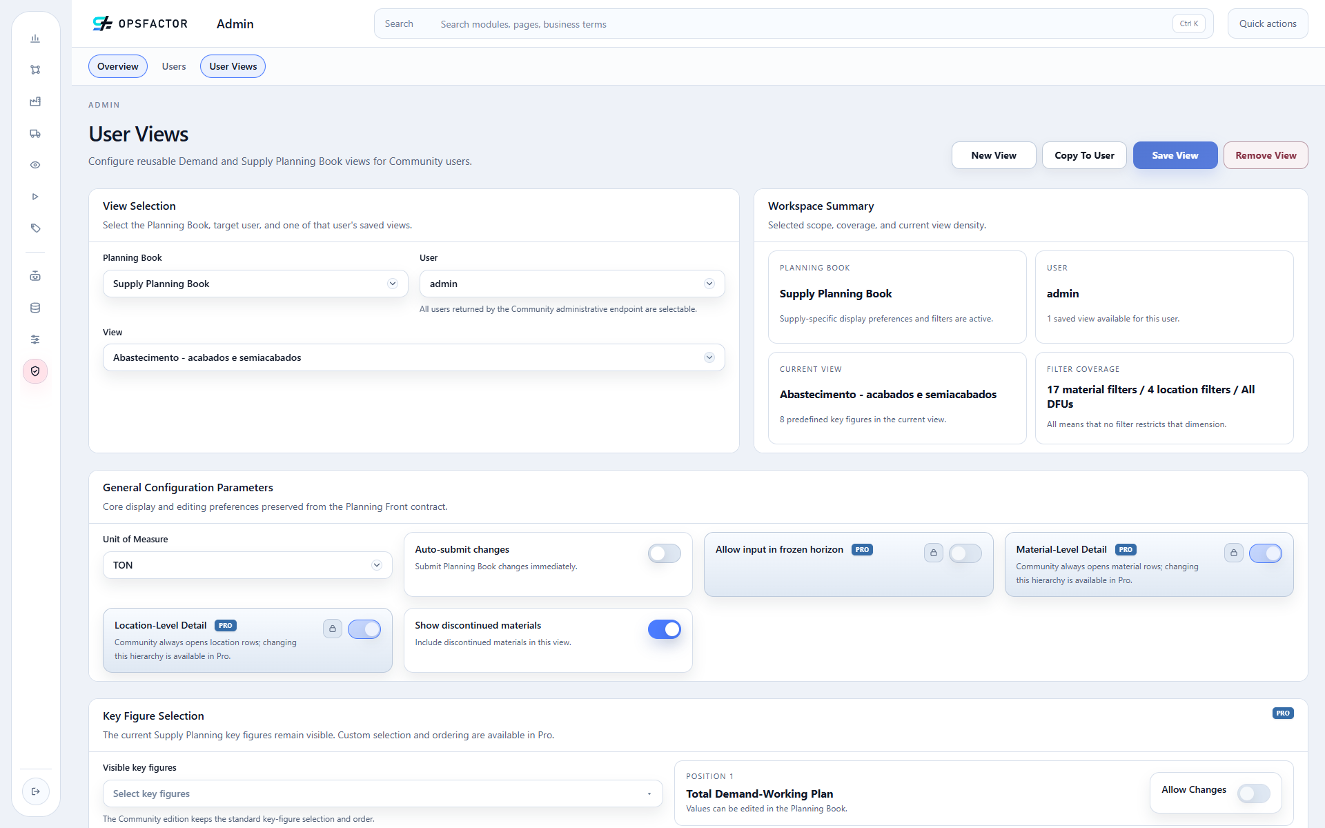
In Admin > User Views, create a Supply Planning Book view named
Abastecimento - acabados e semiacabados for the current user. Select TON,
the ten PA_ materials, three BOBINA_ materials and four PILHA_ materials;
exclude MP_CELULOSE. Select FABRICA_LESTE, FABRICA_SUL, CD_LESTE and
CD_INTERIOR. Community keeps the eight standard measures listed above,
with the -Working Plan suffix; custom selection and ordering are unavailable
in this edition. Check the filters and click Save View. This analysis
does not require editing any planning cell.
Open Supply Chain Planning > Planning Book, select plan 6, this view
and FABRICA_LESTE. Filter to PA_COPIA_A4. Inspect receipts through
Planned Production and Planned Inbound, and requirements through
Direct Demand and Indirect Demand. Indirect demand represents downstream
consumption/supply requirements; it does not prove that a physical outbound
movement occurred. Community has no selectable Planned Outbound row in this
view: use the distribution file to inspect origin, destination and dates.
| PA_COPIA_A4 / FABRICA_LESTE / January 2027 | TON |
|---|---|
| Opening stock | 0.000000 |
| Planned Production | 123.791417 |
| Planned Inbound | 0.000000 |
| Direct Demand | 0.000000 |
| Indirect Demand / Total Demand | 123.791417 |
| Displayed Stock | 0.000000 |
| Production minus requirement | 0.000000 |
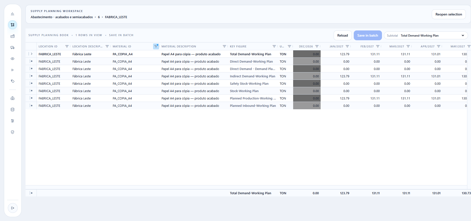
This selection closes the January constrained physical balance: production and distribution outbound both total 123.791417 TON, with no opening stock or receipts. The unconstrained series still shows 161.676010 TON of production and requirements, a 37.884593 TON gap to investigate. Check the three destinations in the distribution export before drawing a customer service conclusion. Zero Safety Stock at the factory is expected: the five-day policy applies to finished goods at the two DCs, not the factories.
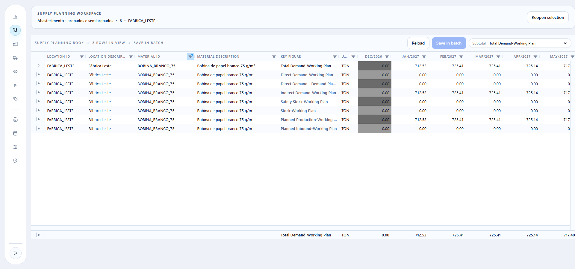
For comparison, select semi-finished material BOBINA_BRANCO_75 at the same
factory. January production and indirect requirements both equal
712.533229 TON, with no inbound and zero opening/closing stock. This local
balance closes. The requirement comes from subsequent production stages,
not direct sales of the roll.
Keep checking the balance after reconciliation
The calculation now reduces flows and fulfilled demand when constrained production cannot cover the requirement. Continue checking receipts, outflows and stock for each material-location-period; a non-negative displayed stock value alone does not prove the entire network feasible.
Check the policy where it actually applies
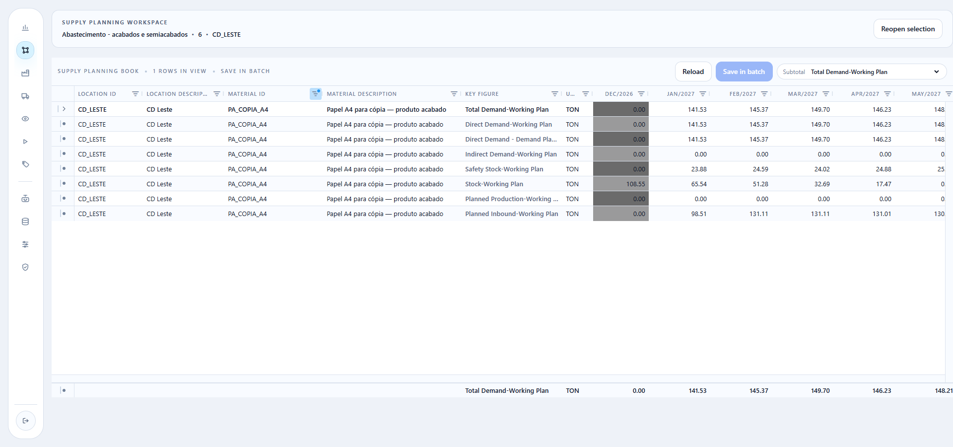
Keep PA_COPIA_A4 and switch to CD_LESTE. January closes as follows:
108.554001 + 98.514201 − 141.529480 = 65.538722 TON
(opening stock + inbound − direct demand = closing stock).
Safety Stock is 23.880621 TON. Closing stock of 65.538722 TON is
above that five-day minimum and below the 85.970237 TON maximum. After
constraints, it need not match the maximum target. Check Maximum Stock Quantity in the original
inventory file to complete the Min/Max review. December returns a zero target
and stock at the horizon boundary; this does not establish coverage beyond
the planning horizon.
To identify non-adherence, filter material-location-period rows where
Projected Stock - Working Version is below Safety Stock Quantity, in the
same unit. This export has 142 rows below the minimum across the reported
material-location-period combinations. Inspect the dimension and month before
assigning the cause to a production resource: a stock target may yield to
preserve physical feasibility. If a row has zero stock and a positive target, record it as a
policy shortfall rather than replacing it with zero.
8. Interpret the fulfilled-demand export
Group Unconstrained Demand, Fulfilled Demand and Unmet Demand by
material, demand location and period, preserving Unit of Measure Id.
Calculate the aggregate rate as total fulfilled divided by total unconstrained
demand; do not average Fulfillment Rate. A zero-demand group has no
calculable fulfillment rate.
The plan 6 file reports 23,857.613389 TON unconstrained, 21,010.483040 TON fulfilled and 2,847.130350 TON unmet: approximately 88.07% aggregate fulfillment. Here the finished-goods production gap matches unmet demand, but the two indicators measure different things. Inspect destinations and periods before generalizing that equality to other plans.
9. Record a supported conclusion
For the selected exception, record the plan, material, location, period and unit; the unconstrained and constrained quantities; the resource or flow evidence; and the effect observed at the destination. Separate facts from an unconfirmed cause.
A useful conclusion identifies the next scenario to test: different capacity, another eligible production version or origin, revised lead time, or a changed inventory policy. Changing those inputs requires a new calculation before claiming that the problem is resolved.
Completion criteria
Complete the review when the extracts use one Supply Plan, finished-goods totals are reconciled without intermediate-stage double counting, one production gap has been traced through occupation and material flows, and the inventory result has been checked at the destination. Explain remaining uncertainties explicitly rather than treating execution status as acceptance.
Return to plan execution, the Supply Planning track, or the course map.