1. Segment markets and demand
What you will build
Split municipality, service rule, and CIF/FOB without duplicating demand.
Before starting
Have materials, municipalities, historical or projected demand, periods, and units defined. Agree on commercial segmentation before introducing sourcing alternatives.
One municipality may contain markets with different requirements. Small retailers and customers needing frequent, fast, or small deliveries may require service exclusively through a DC. Distributors, some industrial segments, and exports may prioritize cost and efficiency, with service from a plant or HUB. These are segmentation hypotheses: each market's rule must reflect actual service commitments and operating requirements.
A customer location can represent a municipality × service segment without being an individual address. For example:
| Demand location | Eligible origins | Reason |
|---|---|---|
| Municipality A / served through DC | Approved DCs | Service requirement |
| Municipality A / served through plant or DC | Authorized plants, HUBs, or DCs | Flexibility to compare service and cost |
If a segment must be served exclusively by a plant, represent that constraint with its own location and eligible lanes. Segment names aid interpretation; network connections and settings enforce the rule. Do not enable an incompatible origin merely because it is nearby.
Allocate CIF and FOB
In this model, CIF identifies demand for which the company pays delivery freight; FOB identifies demand for which the customer bears that leg. Demand must specify how much follows each path, by material and period. The optimizer must not freely convert a CIF sale into FOB to reduce cost.
The following extract was checked against demand in the demonstration
scenario: municipality MUN-2362, material MAT-052, year 2026, and
unit TON. Names and values belong to the anonymized scenario. This is an
explanatory table derived from its records; complete datasets are not distributed.
| Location | Service rule | Demand in TON | Delivery freight to model |
|---|---|---|---|
MUN-2362-CD-CIF |
DC-only / CIF | 5,502.233333 | Less-than-truckload freight table |
MUN-2362-CD-FOB |
DC-only / FOB | 1,218.883333 | Explicit zero cost |
MUN-2362-FAB-CIF |
Plant or DC / CIF | 7,042.666667 | Table for the eligible transportation leg |
MUN-2362-FAB-FOB |
Plant or DC / FOB | 6,448.000000 | Explicit zero cost |
| Total | Municipality × material × year | 20,211.783333 |
The technical suffix FAB identifies the plant or DC segment; it does
not require a plant origin. Check eligible origins in transportation lanes.
Values are shown to six decimal places; reconcile using the records' original
precision before rounding.
Use historical or projected shares for each market. Where origins are flexible,
use the plant or DC segment in the CIF/FOB splits as well and enable both
alternatives. Reconciliation is mandatory: the sum by municipality, material,
and period must equal the original demand without duplication. Also check
prices and other data tied to the customer location.
FOB sets only the customer delivery leg to zero for the company. Plant → DC transfers, handling, and other internal costs remain whenever that path is used.
Find the segments in the interface
- Open Supply Network Explorer and select MALHA-BASELINE.
- Open Location and search for
MUN-2362. Check the four demand locations with theCD-CIF,CD-FOB,FAB-CIF, andFAB-FOBsuffixes. - Distinguish
MUN-2362-GERAL-BASE: it is a reference municipality location, without its own demand in this scenario. Do not duplicate segmented volume there.
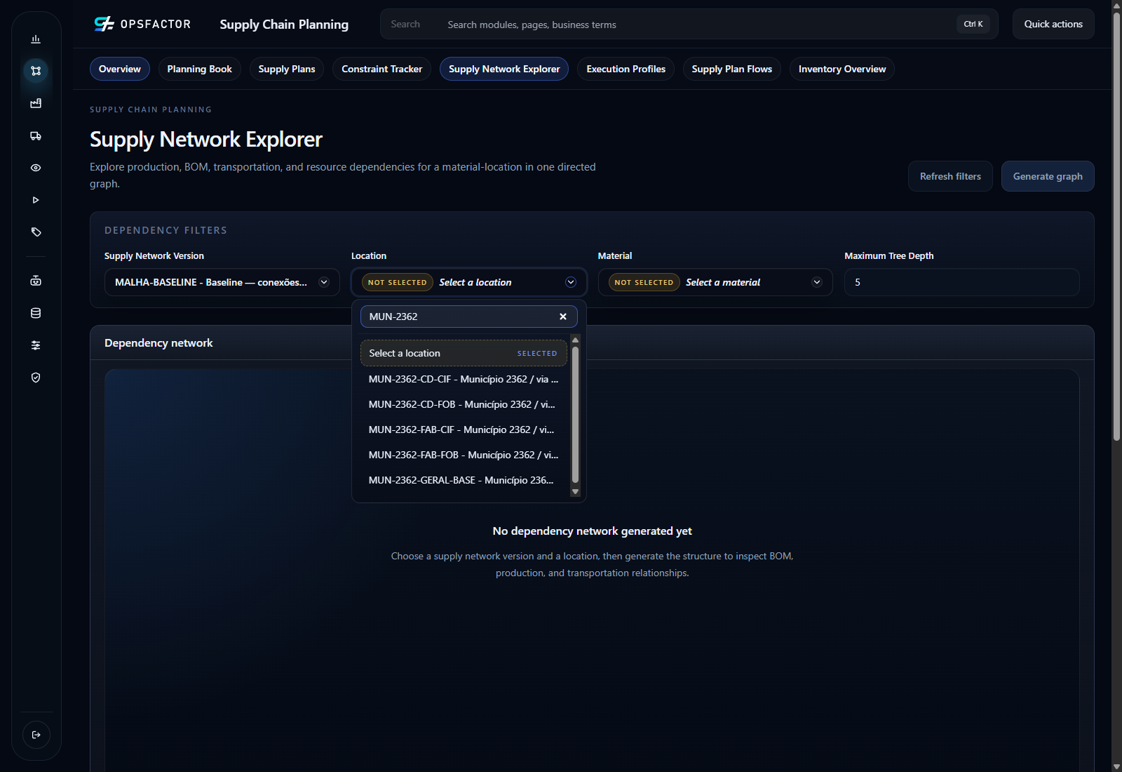
Prepare the demand records
- Separate each municipality's total by material and period. Preserve this total as a control before splitting service segments.
- Determine service and CIF/FOB shares from history or the approved projection. Apply each share to its corresponding total; do not reproduce the entire demand at every new location.
- Create a distinct identifier for each required combination. Use readable descriptions and characteristics that let you filter municipality, service rule, and freight condition without searching for words in names.
- Assign each demand share to its location. Also check prices and other commercial data at the same material, location, and period grain. A share without history must not automatically inherit another share's proportion.
- Add all shares again and compare with the first step's control. In the demonstration extract, the control is 20,211.783333 TON. Reconcile by municipality, material, and period before continuing to freight costs.
Characteristics help select the study's demand scope, including in barycenter analysis. Eligible lanes, prepared in chapter 3, enforce the origin rule. Check both: labeling a customer DC-only without restricting its connections leaves the model incomplete.
Check before continuing
The splits sum to original demand by municipality, material, and period. Each location has an unambiguous service rule and CIF/FOB category; allowed origins reflect these rules.
Previous: Training map.